Geographically weighted regression for spatial analysis in BigQuery

Although leading data warehouses already offer some level of support for spatial data they can usually only work with core spatial functionalities and lack some of the advanced analytical capabilities required for many geospatial use cases. The CARTO Analytics Toolbox extends the geospatial capabilities of the most popular cloud data warehouses using spatial SQL which means both easier integrations as well as accessibility  given SQL’s universal adoption within the spatial community. Our Analytics Toolbox already unlocks more than 60 advanced spatial functions using a set of User Defined Functions (UDFs) and procedures covering a broad range of spatial use cases  including: data transformations  spatial indexing and advanced functions to carry out geocoding  clustering  route calculations  and more.

As part of the Advanced modules for Google BigQuery, we have now added support for the Geographically Weighted Regression (GWR) method  a statistical regression method that models the local (e.g. regional or sub-regional) relationships between a set of predictor variables and an outcome of interest.

Suppose we have data across the whole UK on the number of crimes per area as well as other associated variables (i.e. such as the unemployed active population or the level of urbanity of the area) and we wanted to model the number of crimes as a function of such variables. The output from this regression model would be a set of parameter estimates  each reflecting the relationship between the number of crimes and a particular attribute. The parameter estimates in this scenario are global statistics and describe the average relationship for the whole of the UK  which is assumed to be a good representation of any local relationship across the territory.

However  the global relationship might hide local differences as well as contrasting relationships in different parts of the study area which tend to cancel at the global level. In other words  there might be particularities in the relationship of the different variables in specific areas of the country (e.g. Central London, Manchester area  rural areas) that may get cancelled if we only study the behaviour in an aggregated manner.

GWR is an exploratory method that allows us to detect spatially-varying relationships between the variable of interest and any relevant attribute. It works by moving a weighted window over the data, estimating one set of coefficient values at every chosen fit point.

This technique involves either choosing (or selecting by leave-one-out cross-validation) a bandwidth for an isotropic spatial weights kernel and for each data point run a weighted regression based on this kernel, such that for location "i" the other observations are weighted in accordance with their proximity to "i."

In this blogpost we will showcase how to use the GWR method available in the CARTO Analytics Toolbox by analyzing the local relationships in the UK for two use cases: the first  will look at the local variations of the association between the number of crimes per population and the unemployed active population and the average house price  while the latter will model the local relationship between the net annual income and the likelihood to smoke.

GWR is now available in the CARTO Analytics Toolbox

The current implementation of the GWR method available in the Analytics Toolbox takes advantage of spatial indices to construct the neighborhood matrix: using the kring function in fact we can easily find for any grid cell the neighbouring cells for a different order of neighbors. The procedure available in the Analytics Toolbox also allows the user to specify the type of kernel used to construct the neighborhood matrix: uniform  triangular  quadratic  quartic and gaussian.

To test the procedure  we used the GWR method to estimate the local relationship between the number of crimes per 100 000 population in the UK and the number of unemployed economically active population and the average house price. This data is provided by our partner Doorda at the Output Area (OA) level and it is available as a premium dataset via the Data Observatory. To use the GWR procedure first we need to transform the data into one of the supported spatial indices  either H3 or the Quadkey grid.

The following query, which also takes advantage of the data enrichment functionality available in the Analytics Toolbox, was used to project the data at the OA level to an H3 grid with resolution 7 either by area interpolation of the H3 grid cells with the OA geometries (for extensive variables  e.g. the average house price) or by sum (intensive variables, e.g. the number of crimes  the total population  and the economically active unemployed population):

CALL `carto-un`.data.ENRICH_GRID(
   'h3' 
   R'''
   SELECT *
        FROM UNNEST((SELECT `carto-un`.h3.ST_ASH3_POLYFILL(
            ST_GEOGFROMTEXT('POLYGON ((-9 50,  4 50, 4 62,  -9 62,  -9 50))'),  7)
        )) as h3id
   ''', 
   'h3id', 
   R'''
   SELECT geom  
           crime,  pop,  economically_active_unemployed all_average_price
           FROM `myproject.mydataset.doorda_oa`
   ''', 
   'geom', 
   [('crime',  'sum'), 
   ('pop',  'sum'),  
   ('economically_active_unemployed',  'avg'),  
   ('all_average_price',  'avg')
    ], 
   ['`myproject.mydataset.doorda_h3`']
);

where myproject.mydataset.doorda_oa and myproject.mydataset.doorda_h3 are respectively the input and output tables in Google BigQuery  and the H3 index (h3id) is obtained for a polygon that encompasses all of the UK area.

With the data transformed into an h3 grid  we can now run the GWR_GRID method:

CALL `carto-un`.statistics.GWR_GRID(
    'myproject.mydataset.doorda_h3',  
    ['economically_active_unemployed_std', 'all_average_price_std'],  
    'crime_pop_100k',  
    'h3id',  
    'h3', 
    6,  
    'gaussian',  
    True,  
    'myproject.mydataset.doorda_h3_gwr'
);

where we used a Gaussian kernel with a kring distance of 6  which corresponds to a distance of order of neighboring cells of 6, and we have standardized all the covariates.

As a result we obtain the local estimates for the model coefficients, which are shown in these maps:

with positive (negative) values indicating a positive (negative) association between the number of crimes per 100,000 population and the corresponding predictor (conditional on the other) and with larger absolute values indicating a stronger association.

We can see that overall  after accounting for the average house price, where the economically active unemployed population is higher, the number of crimes per population is also higher. However  the strength of this association is weaker in the largest metropolitan areas (London  Birmingham  and Manchester). On the other hand  conditioned on the active unemployed population  the association between the number of crimes and the house price does not show a clear pattern. We can also compare these results with the output from a global regression model:

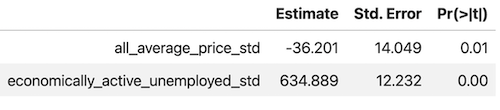
From this table, we can see that the results of a global regression model can be misleading  as they indicate a positive (statistically significant) association between the crimes per population and the economically active unemployed population while the local analysis shows that this association varies indeed with space. On the other hand  conditional on the economically active unemployed population  the association with the average house price is not significantly at the 0.01 level in the global model  which can be explained by both positive and negative values of the local coefficients.

Similarly  we can look at the relationship between the net annual income and the likelihood of being a smoker. If we look at the global estimates:

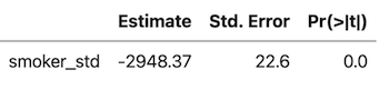
We see that there is a statistically significant negative relationship between income and the likelihood to smoke. However  when looking at the local estimates as derived from a GWR model:

We see that overall the strength of this association is weaker in some areas  such as part of the London area and in some northern cities.

Enhance your spatial analysis in SQL with CARTO Analytics Toolbox

As of today, the GWR method is available in our Spatial Extension for BigQuery. We will be announcing further cloud native developments in the coming weeks, so stay tuned for regular updates from us!

Want to get started?

Sign up for a free 14-day trial

This project has received funding from the European Union's Horizon 2020 research and innovation programme under grant agreement No 960401.