Getting Started with SQL in CARTO

CARTO is built on a database called PostgreSQL. The SQL part of that means structured query language, which is a powerful and popular language for analyzing tables of data. It is based on mathematics called relational algebra, which has a solid foundation.

SQL queries work on data arranged in tables that are visually similar to an Excel spreadsheet, but have very different underlying mechanics. Table names are lowercase, contain no spaces, and are unique within a CARTO account. Tables have columns that have headings that are all lowercase with no spaces. Column names cannot be the same as some of the keywords in SQL.

In this lesson, we will be using CARTO to discover some of the basic features of SQL and introduce the geospatial extension called PostGIS. PostGIS allows you to perform geospatial queries such as finding all data points that are within a given radius, the area of polygons in your table, and much more.

Let’s get started exploring SQL by working with our familiar dataset on earthquakes. You can easily import it by copying the following link and pasting it into the CARTO Importer:

  https://carto.com/academy/d/all_month.csv.zip

If you prefer to have up-to-date earthquake data, go to the USGS site and grab the “all earthquakes” data for the past 30 days.

After your data is successfully imported, rename the table by clicking on the dataset name in the upper left and typing in earthquake_sql. After you have done this, inspect the columns you have in your table. Each column has a unique name, and the columns of data are imported as one of five types:

• number – 1, 3.1415, -179.3, etc. using double precision floats
• string – a string of characters, e.g., “Socotra archipelago”
• boolean – true or false
• date – date and time
• geometry – associates your data with geographical coordinates

In addition, a cell without data entered will be shown as null. Notice also that rows represent unique entries defined by their cartodb_id.

SELECT, *, and FROM

Once you have finished inspecting your data, click on the tab on the right labeled SQL. This gives you a view of a basic SQL statement.

Notice the words in the text editor:

• SELECT – choose the columns specified after SELECT
• * – a wildcard that means all columns in a table
• FROM – this is needed to specify from which table the data is pulled

Using the above list as a guide, the statement in the SQL tab, SELECT * FROM earthquake_sql, reads: “Select all columns from the table earthquake_sql.” The order of your SQL query matters. For example, the FROM statement needs to come after your column list. If you were not interested in having all of the data in your table, you could write a comma separated list of the columns you are interested in instead. For instance, if you only care about the location (the_geom), the magnitude (mag), and where the earthquake occurred (place), then your SQL statement would read as:

SELECT the_geom, mag, place
FROM earthquake_sql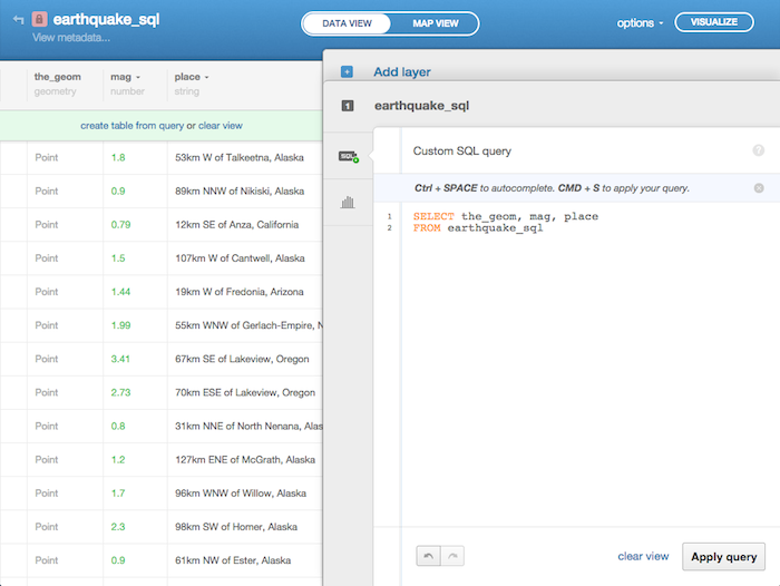

When you run this query by clicking the button “Apply query”, or typing CMD+S (Mac)/CTRL+S (PC), you are presented with the option “create table from query” that allows you to create a new table from your SQL statement. If you choose this, you create a new data table that can be used independently of the current one. If you instead want to revert to having all the columns that you previously imported, clicking “clear view” returns your SQL statement to SELECT * FROM earthquake_sql and you see all of your data in the table again.

Tip: You may have noticed that if you run the above query, the data disappears from your map. You’ll soon find out the reason for this in the section below on the_geom_webmercator.

Our basic format for a SQL statement is:

SELECT columns
FROM table_name

Pro Tip: If you want to rename a column when you create a new table from query, you would write: column_name AS new_name. If you wanted to change mag, you would put mag AS magnitude into your SELECT statement. The ‘AS’ keyword gives the old column name a new alias. Also note that this does not actually change anything in the original table–it just creates a new temporary table with the new information that you selected. We will explore methods for updating tables in the coming lessons.

Filters show us WHERE…

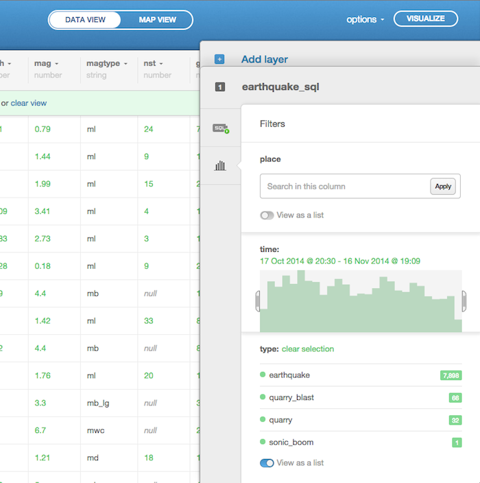
Still in the Data View, check out the tab below the SQL tab, the one that has a bar graph. This is our Filters tab.

Filters in CARTO are an excellent way to explore your data because they help you analyze the contents of columns by showing, depending on the characteristics of the data in the column, the unique entries, a histogram of the data distribution, or the range in values of another column. For instance, it may not be obvious to expect that quarry, quarry_blast, explosion, or sonic_boom are possible entries that can exist alongside of earthquakes in the type column.

Start by exploring the options available when you apply the filters to your data. Look specifically at different columns of data and how you are presented with distinct methods for filtering.

Things to notice:

• Filtering by place only lets you search for strings because of the large number of unique, non-numerical entries
• Filtering by type gives you a list of a few values because there are only a few unique entries
• Filtering by time allows you to select a range in time
• Filtering by gap gives you a histogram of the values in that column

Behind the scenes, these filters are setting up SQL statements that are run against our data. To see how the data table changes in response to your filtering, change the sliders, enter search terms, etc.

Once you’ve finished exploring your data with filters, remove all of the filters by clicking the grey circle with an × in the top right of each window’s pane. Then re-add the filter for type, deselect all entries except earthquake and quarry, and switch to the SQL tab to see what your filtering produces for a SQL statement.

As you will see, filters show us the WHERE clause that allows you to select rows based on criteria you set. In this case, the WHERE clause chooses all rows that have either “earthquake” or “quarry” in the type column. That is, a row is only chosen if type matches “earthquake” or “quarry”.

We could easily flip this condition around by placing the ‘NOT’ keyword before ‘IN’, and we would only get all rows that do not have “earthquake” or “quarry” in the type column.

Delete all of the text after WHERE, and type cartodb_id = 4. Once you finish typing, apply the query and inspect the results. As you will see, all records that do not have a cartodb_id of 4 disappear from view. You can apply other conditions, such as cartodb_id > 2 or even on-the-fly calculations such as cartodb_id * 2 > 4.

Switch back to the Filters tab, hit “Clear view” to clear the last SQL command, and add an additional filter. This time choose depth, then select a range and switch back to the SQL tab. We can discover that we can use the following inequalities:

• > for greater than
• < for less than
• >= for greater than or equal to
• <= for less than or equal to
• <> or != for not equal to

We also discover that we can chain conditions together using the ‘AND’ keyword. In the case of our depth filter, you have the following format:

  depth <= value1 AND depth >= value2

If you add another filter you can see that they are all chained together to give a more nuanced selection of your data. The ‘OR’ keyword is another option for having multiple conditions.

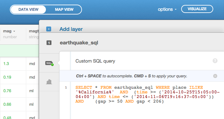
The final condition we will discover through our filters can be found by filtering place. Clear all filters except for place. Type in “California” and then switch to the SQL tab. You will see a new keyword ILIKE that does basic regular expression matching that is case-insensitive. If you want case-sensitive matching instead, you need to use LIKE.

To avoid confusion with the * in the SELECT statement, the wildcard that is used for pattern matching with LIKE and ILIKE is the percent symbol: %. Placed at the front of the string, place ILIKE '%california', matches all strings that end in “California”, regardless of case. Placed at the end, 'california%', matches all strings that begin with “California”. Placed on both ends, '%california%', as produced by the filter, it matches all strings that contain “California”.

While % matches a sequence of zero or more characters, the underscore (_) matches any single character. The following will match “California”: '_a_i_o_n_a'.

Tip: Make sure to use single quotes (‘) to enclose strings in the WHERE clause.

We now have a larger view of what a query can look like:

SELECT columns
FROM table_name
WHERE conditions

ORDER BY and LIMIT

Another way to inspect your data is by ordering the columns of the table differently. CARTO has automatic ordering built in–just click on a column name and select ASC or DESC to get the data ordered how you want. ASC orders your data by lowest number or highest in the alphabet (closest to A) first, while DESC does the opposite.

You can perform the same operations using the SQL keywords ORDER BY. Try it out by first clearing your view and then, after your table name, typing:

ORDER BY depth ASC

This will arrange your data in your table to be ordered by the depth column. The result has no effect on how the data is displayed in CARTO unless you apply other keywords to your overall SQL statement.

Pro Tip: You can add multiple columns after the ORDER BY keywords. The first column is sorted first, then within that ordering the second column is ordered, etc. It goes like this:

SELECT *
FROM table_name
ORDER BY column1 ASC, column2 DESC

One keyword that changes the display of data on your map depending on the ordering is LIMIT, which gives you the number of rows requested if there are that many to display. This is added to the end of your SQL statement:

SELECT columns
FROM table_name
WHERE conditions
ORDER BY column_name
LIMIT N

where N is an integer from 0 to however many rows your table contains. If you want ten rows to display, you will type LIMIT 10. This is useful if you want to display a simplified version of the data on your map.

Also note that while our SQL block keeps growing, WHERE, ORDER BY, and LIMIT are optional.

If you have any SQL applied, click on the “Clear view” option to reset your query.

the_geom

Now that we have a handle on some basic SQL, we will shift our focus to two special columns in CARTO. The first is the_geom, which is where some of your geospatial data is stored. If your data does not have latitude and longitude, or other complicated geospatial data types such as lines, polygons, etc., then you can try geocoding to obtain them. Since our earthquake data comes with latitude and longitude already, CARTO knows at import to read these into the the_geom column.

Start by double-clicking on a cell in the the_geom column. In the resulting menu, click the toggle next to “Geometry.” You will notice that data is structured like the following:

{
  "type": "Point",
  "coordinates": [-120.5188, 49.4037]
}

While the underlying geometry is in a different format, this data has been translated to GeoJSON. In our case, we have a point type geometry with coordinates at the values listed. Note that longitude is first and latitude is second, similar to (x,y) from plotting in a Cartesian coordinate plane. Just like there are different coordinate systems besides Cartesian (e.g., polar, spherical, etc.), maps have different coordinate systems, or projections. The_geom is stored in a system called WGS84. Hear more about all of it’s beautiful intricacies from this great video.

the_geom_webmercator

The other geospatial column that CARTO uses is the_geom_webmercator. This column contains all the same points that were in the_geom, but projected to Web Mercator, a web-optimized version of the historical Mercator projection. The_geom_webmercator is required by CARTO to display information on your map. It is normally hidden from view because CARTO updates it in the background so you can work purely in WGS84. You can easily inspect it by typing the following SQL/PostGIS statement into the text editor in the SQL tab:

SELECT cartodb_id, ST_AsText(the_geom_webmercator) AS the_geom_webmercator
FROM earthquake_sql

As you can see, the values range from around -20 million meters to +20 million meters in both the N/S and E/W directions because the circumference of the earth is around 40 million meters. This projection takes the furthest North and South to be ± 85.0511°, which allows the earth to be projected as a large square, very convenient for using square tiles with on the web. It excludes the poles, so other projections will have to be used if your data requires them.

Also note a new type of object appearing in the SQL statement above: ST_AsText(). This is a PostGIS function that takes a geometry and returns it in a more readable form.

There are many variants to the common projections, so groups of scientists and engineers got together to create unambiguous designations for projections known as SRID. The two of interest to us are:

• 4326 for WGS84, which defines the_geom;
• 3857 for Web Mercator, which defines the_geom_webmercator.

We will find out how to use these in the section below and in future lessons.

Basic PostGIS usage

In this section, we are going to just get our feet wet with PostGIS. Like we did with the data we’ve encountered so far, spatial data can be manipulated, filtered, ordered, and measured in a database by using the geometry in the_geom or the_geom_webmercator.

The functions that allow us to do this come out of PostGIS and all begin with “ST_”, just as we saw with ST_AsText() above. CARTO also introduces some helper functions that reduce the amount of typing on the user’s end. These begin with “CDB_”. For example, we will use CDB_LatLng(lat,long) to get a coordinate in the 4326 projection (WGS84).

We’ll keep working with the earthquake data, but trying to generate some new useful information from it. Say you are interested in knowing the distance in kilometers your office is from all of the earthquakes in the data table. How would you go about doing this?

First you would need to know your location. Let’s say you’re in downtown San Francisco, which is near (37.7833° N,-122.4167° W), so we can just use the CDB_LatLng() function to generate the proper geometry.

Introduction to Measurements

Next we need to find a PostGIS function that allows us to find the distance we are from another lat/long location. Looking through the PostGIS documentation, you will find a function called ST_Distance() that has the following function prototypes:

float ST_Distance(geometry g1, geometry g2)
float ST_Distance(geography gg1, geography gg2)
float ST_Distance(geography gg1, geography gg2, boolean use_spheroid)

This function is overloaded, meaning that we have multiple options for the input variables we can pass to it. Before using it, though, we should look at what the arguments mean:

• geometry type arguments: allows you to measure the distance in degrees (lat/long)
• geography type arguments: allows you to measure the distance in meters
• use_spheroid argument: use WGS84’s oblate spheroid earth (pass true) or assume the earth is perfectly spherical (pass false)

Two things to notice about this function. First, we cannot mix projection types. For example, you cannot measure the distance between a value in the_geom and a value in the_geom_webmercator. Second, the function returns a float point data type that is a measurement in the same units as the input projection.

Measurement Units

What does that mean, measurement in the same units as the input projection? Well, it is a funny thing. Let’s say you want to measure the distance between two points stored in the_geom that we can call the_geom_a and the_geom_b. If you input them both into ST_Distance(the_geom_a, the_geom_b) the result would come back in units of WGS84. This is not very useful because the answer is in degrees. Instead, we want to measure distance in meters (or kilometers).

You can measure distances (and make many other measurements in PostGIS) using meter units if you run the measurements with data on a spherical globe. That means we can exclude the first version of ST_Distance(). Instead, we need to project the_geom and our point to PostGIS geography type. We can do this by appending ::geography to both of them in the function call, as below. Notice that we need to divide the value returned by ST_Distance() by 1000 to go from meters to kilometers.

SELECT
  *,
  ST_Distance(
    the_geom::geography,
    CDB_LatLng(37.7833,-122.4167)::geography
  ) / 1000 AS dist
FROM
  earthquake_sql

The spaces and new lines are added to make it more readable. SQL is very forgiving about whitespace, so it will run as printed. This query produces the table you will be needing for the next section.

Pro Tip: In spatial functions, if an option is available that includes the boolean use_spheroid option, it will achieve the same result as casting your results using the ::geography method. You could use it as follows:

ST_Distance(the_geom, CDB_LatLng(37.7833,-122.4167), true)

To test it out, run the following SQL to look at the average and standard deviation of the difference between the two calculations–both should be zero. The code block scrolls to the right.

SELECT
  AVG(ST_Distance(the_geom::geography,CDB_LatLng(43,-122)::geography) - ST_Distance(the_geom,CDB_LatLng(43,-122),true)) as average,
  STDDEV(ST_Distance(the_geom::geography,CDB_LatLng(43,-122)::geography) - ST_Distance(the_geom,CDB_LatLng(43,-122),true)) as std_deviation
FROM earthquake_sql

Pro Tip: Aggregate functions such as AVG() and STDDEV() are functions that use multiple rows to make a calculation. You can find their documentation at the PostgreSQL website.

Mapping with SQL results

Once you successfully run your query from above, save the result as a new dataset. It is now easy to make a graduated color map by using the new dist column to give a visualization of earthquakes in proximity to San Francisco.

That’s it for Lesson One of SQL and PostGIS in CARTO.

Want more? Check out some tutorials:

• Query by distance
• Counting points in polygons