Intersect and Aggregate
Apply the Intersect and Aggregate analysis to count the number of points that intersect in a polygon.
This guide provides an example of how to apply the Intersect and Aggregate analysis option to count the number of points that intersect in a polygon.
If you were applying SQL code, you would have to create a new column in your polygon dataset and apply a SQL query to store and visualize the number of points in each polygon. With Builder, this is easily applied by adding the Intersect and Aggregate analysis option directly to the map layer.
Import CARTO File
For this example, we will analyze which borough in NYC has the largest number of rat sighting complaints on 311.
-
Import the template .carto file packaged from the “Download resources” of this guide and create the map.
Click on “Download resources” from this guide to download the zip file to your local machine. Extract the zip file to view the .carto file(s) used for this guide.
Builder opens displaying a Rat Sightings as the first map layer and NYC boroughs as the second map layer. The datasets used in this dashboard are:
-
Polygon layer of New York City boroughs (
ny_boroughs) from the Data Library. -
Point data for 311 complaints about rat sightings in New York City from NYC Open Data.
-
-
Double-click on
ny_boroughsand rename the map layer to Boroughs.
Count the Points that Intersect in the Polygon
Apply an analysis to count the number of rat sightings that intersect in each borough.
-
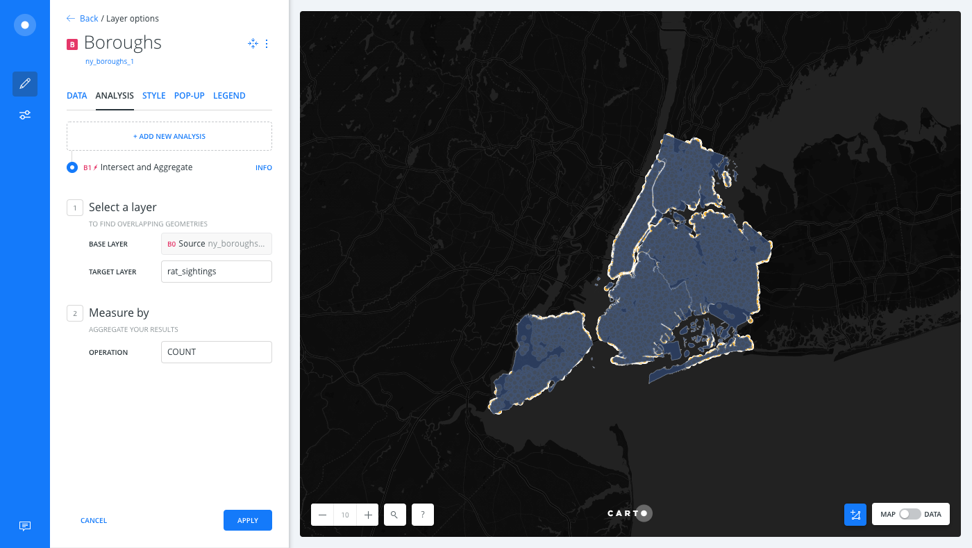
From the Boroughs map layer, click the ANALYSIS tab.
-
Click ADD ANALYSIS and apply the following Intersect and Aggregate options:
- For the INTERSECT LAYER, select the Rat Sightings map layer.
- For OPERATION, keep the default Count.
- Click APPLY.
Analysis Columns
As a result of the analysis, two new columns are created. count_vals represents the total count of rat sighting incidents in the boroughs, and count_density is the density of rat sightings in each borough.
CHEATSHEET: count_vals and count_vals_density
If you are applying multiple Intersect Second Layer analyses, the analysis result columns count_vals and count_vals_denstity append a number suffix to the columns to differentiate between each analysis node.
For example, if two concurrent COUNT analysis are applied to a layer, the analysis result generates a count_vals and count_vals_density column for analysis node A1. For the second analysis node A2, the analysis generates count_vals_2 and count_vals_density_2 columns.
Intersect with second layer oftentimes is a Point in Polygon calculation, which counts the number of incidents in a polygon. Raw count values can be misleading because counts could have a population density dependence.
To cancel this effect, this analysis returns one normalized version of the count variable: count_vals_density. This quantity is the counts divided by the polygon area. Another step could be to add an Enrich from Data Observatory analysis to get the total population, then divide the count output by this population.</ul><ul>See the Enrich from the Data Observatory guide for more information.</ul>
Style the Analysis Results
Style the map layer By Value to visualize the results of the analysis.
-
From the Boroughs map layer, click the STYLE tab.
-
Click the By Value option for POLYGON COLOR.
-
Select the
count_valscolumn. A default color scheme is applied.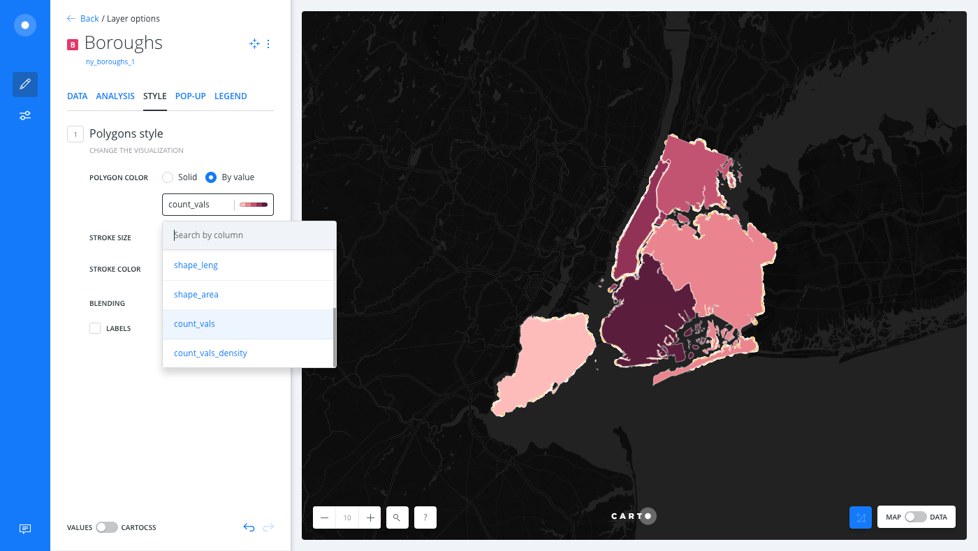
-
Switch the slider button, located at the bottom of the STYLE tab, from VALUES to CARTOCSS and apply the following custom styling.
 #layer {
   polygon-fill: ramp([count_vals], (#123f5a, #2b6c7f, #559c9e, #8eccb9, #d2fbd4), quantiles);
   polygon-opacity: 0.7;
   line-width: 0.1;
   line-color: #f4f0f0;
   line-opacity: 0.5;
   polygon-comp-op: multiply;
 }

 #layer::labels {
   text-name: [boroname];
   text-face-name: 'DejaVu Sans Book';
   text-size: 12;
   text-fill: white;
   text-label-position-tolerance: 0;
   text-halo-radius: 1.2;
   text-halo-fill: black;
   text-dy: 0;
   text-allow-overlap: true;
   text-placement: point;
   text-placement-type: dummy;
 }
Interested in learning about styling with CartoCSS? View the Basic CartoCSS for Map Styling Guide.
-
To enhance the styling even more, go back to the LAYERS list in Builder and apply the following CartoCSS to the
Rat Sightingsmap layer, or download the final .carto file provided from the “Download resources” of this guide to view all of the cartography and widgets applied.
#layer {
  marker-width: 1.5;
  marker-fill: #ffffff;
  marker-fill-opacity: 0.41;
  marker-allow-overlap: true;
  marker-line-width: 0.03;
  marker-line-color: #7e7e7e;
  marker-line-opacity: 0.5;
}
Limits
This analysis has a limit on the time that it takes to execute the analysis. If the analysis takes more than 5 minutes, CARTO will return a timeout error.
External Resources
If you are interested in using the underlying functions in the SQL view of Builder, you can create a new column in your dataset and store the result with a ST_Intersects query. For details, see the PostGIS ST_Intersects documentation.