Relational Joins and Spatial Joins
Joining data in CARTO is a very common task. Not all joins are equal though, and the one you use is going to depend a lot on your data and what you want to create. Here we are going to walk you through some common JOIN methods in CARTO. In each section we will show you how to join the data using SQL on-the-fly and then show you how to write the result of a join into your table.
Join two tables by a shared value in each row
This is the type of join you perform when you have a value in two tables (say country ISO codes) and you want to match rows from one table to the next (e.g. iso_code='USA') from one table with the same value in a second table (e.g. iso='USA'). Column name doesn’t matter, just the content!
table_1
| cartodb_id | the_geom | iso_code |
|---|---|---|
| 1 | Polygon… | USA |
| 2 | Polygon… | BRA |
| 3 | Polygon… | BEL |
| 4 | Polygon… | GAB |
table_2
| cartodb_id | iso | population |
|---|---|---|
| 1 | PBRA | 302 |
| 2 | USA | 188 |
| 3 | GAB | 99 |
| 4 | BEL | 876 |
The above tables give a good example when you will want to use this method. Say you have some nice polygons for your world borders stored in table_1, but you have a CSV with a value you need for your map and you’ve uploaded it seperately to table_2. Here is the join command you would run:
SELECT table_1.the_geom,table_1.iso_code,table_2.population
FROM table_1, table_2
WHERE table_1.iso_code = table_2.iso
You’ll see, it doesn’t matter that the columns in the two tables were different, iso_code versus just, iso, we still ran the join just fine. You could now use Merge with dataset from the Edit drop-down menu to create a new dataset with this data. Otherwise, we can just write it into the first table. Here’s how.
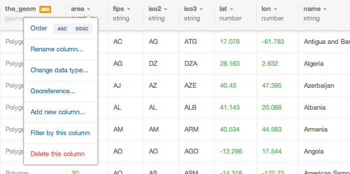
First, create a new column in table_1 called ‘population’ and make it of type ‘number’. You can do this by clicking the drop down arrow at the top of any column and selecting Add new column.
Next, check in table_2 and be sure that under the population column, the type is Number. If it says String, just change it. Click String and then choose Number, and accept the warning. Next run this SQL:
UPDATE table_1
SET population = table_2.population
FROM table_2
WHERE table_1.iso_code = table_2.iso
There is another variation that will do the same thing, but sometimes you will find it simpler to write:
UPDATE table_1 as t1
SET population = (
  SELECT population
  FROM table_2
  WHERE iso = t1.iso_code
  LIMIT 1
)
In the second exampe we run a subquery, so for each row of table_1 it runs the query inside the parentheses. You’ll notice some neat tricks in the example query. We use t1 as an alias for table_1, so we don’t have to write the full name multiple times. We also use LIMIT to make sure that the second query only gives back one result per row, otherwise we might get an error if the second table contained multiple values for some countries. Depending on what your data is, it may not be good to add a LIMIT because you will want to somehow combine all the resulting rows into one answer. If that is your case, keep reading!
Join two tables by aggregating the shared values in a second table
This is the case where you have many values in a second table, and you want to get some collection of their values where a shared column match the first table. Here we are talking about examples such as, SUM, AVG, MIN, MAX, etc. We will do just like we did above, but in this case we use a function to aggregate all values in the second table.
table_1
| cartodb_id | the_geom | iso_code |
|---|---|---|
| 1 | Polygon… | USA |
| 2 | Polygon… | BRA |
| 3 | Polygon… | BEL |
| 4 | Polygon… | GAB |
table_2
| cartodb_id | iso | day | total |
|---|---|---|---|
| 1 | BRA | m | 4 |
| 2 | BRA | m | 5 |
| 3 | BRA | w | 2 |
| 4 | USA | m | 2 |
| 5 | USA | f | 1 |
Here is our new example data. We want to get the sum of all totals in each country. So, the SQL would look like this:
SELECT
  table_1.the_geom,
  table_1.iso_code,
  SUM(table_2.total) as total
FROM table_1, table_2
WHERE table_1.iso_code = table_2.iso
GROUP BY table_1.iso_code, table_2.iso
The biggest change now is the use of the GROUP BY method. This collapses all rows that have a shared ‘iso’ value, and then using SUM it sums up all the values in total from those collapsed rows! Nice, right? Now, lets add a column to table_1 called total and make it numeric. Now to do the update version of the query:
UPDATE table_1 as t1
SET total =  (
  SELECT SUM(total)
  FROM table_2
  WHERE iso = t1.iso_code
  GROUP BY iso
)
Pretty simple. We can do this all day long!
Here are some other types of functions other than SUM you might be interested in.
Join two tables by geospatial intersection!
One of the most exciting joins is done by using geospatial intersections. If you have a set of points in one table, and a set of state polygons with iso_codes in a second. You could use a geospatial intersection to give each point an ISO code based on the state they fall in. We can also of course combine COUNT, SUM, AVG, MIN, MAX and all that good stuff here too! Here is some example data:
table_1
| cartodb_id | the_geom | iso_code |
|---|---|---|
| 1 | Polygon… | USA |
| 2 | Polygon… | BRA |
| 3 | Polygon… | BEL |
| 4 | Polygon… | GAB |
table_2
| cartodb_id | the_geom |
|---|---|
| 1 | -58.299992, -33.989619 |
| 2 | -56.709986, -34.349959 |
| 3 | -56.48602, -30.415987 |
| 4 | -57.599957, -30.259614 |
Let’s say we just want to know the total number of points from table_2 that fall in table_1. Easy, let’s see the SQL:
SELECT table_1.the_geom,table_1.iso_code,COUNT(*) as count
FROM table_1, table_2
WHERE ST_Intersects(table_1.the_geom, table_2.the_geom)
GROUP BY table_1.the_geom, table_1.iso_code
The ST_Intersects function is one you are going to use again and again. You’ll love it. Now, let’s do the same but insert the result into a new column. Start by adding a column to table_1 called total and make it numeric. Next, run:
UPDATE table_1 as t1
SET total =  (
  SELECT COUNT(*)
  FROM table_2
  WHERE ST_Intersects(the_geom, t1.the_geom)
)
Nifty, right? You can now use this in combination with SUM, AVG, MAX and all that good stuff to get the values you need from one table into the next.
Join two tables dynamically
Just a note about doing the above for a map you build on Leaflet. You may not always want to write the result into table_1, instead, you may want to query data live from the browser based on something the user is doing. In those cases, use the SELECT statements. If you are rendering a map with the results, you just need to remember to include the_geom_webmercator is all! It is our hidden reprojection of the_geom that makes the final map speedy. Here is the above query modified to include it:
SELECT
  table_1.the_geom,
  table_1.iso_code,
  COUNT(*) as count,
  table_1.the_geom_webmercator
FROM table_1, table_2
WHERE ST_Intersects(table_1.the_geom, table_2.the_geom)
GROUP BY table_1.the_geom, table_1.iso_code
Join two real datasets
Now, let’s run through an example using a couple real datasets. Start by getting two datasets ready in your CARTO account. To find them, go to your account dashboard. From the Data View, click Data library. Search for the dataset called ‘World Rivers’ and click Connect dataset. This will load the data and take you to the resulting table. If you click on Map view, you’ll see that it is a basic map of some of the worlds large rivers. This comes from Natural Earth Data. Take note of the name of the table that was created, in our case it was table_50m_rivers_lake_cen.
Next, go back to your Dashboard by clicking the back link in the upper left. Repeat the process importing a different table from the Data library. This time you have to import ‘World Borders’ dataset. When the table finishes loading click Map View, and you’ll see that it is a dataset of all country borders. Let’s join the rivers with the countries so we can make a choropleth of the total length of big rivers in countries around the world. Of course, our map is going to ignore all the little rivers not included in our dataset, but this is just an example!
Joining the data
From inside your country borders table create a new column to hold some numerical data. In the Data View, click the drop down arrow beside any regular column name and then click Add new column.
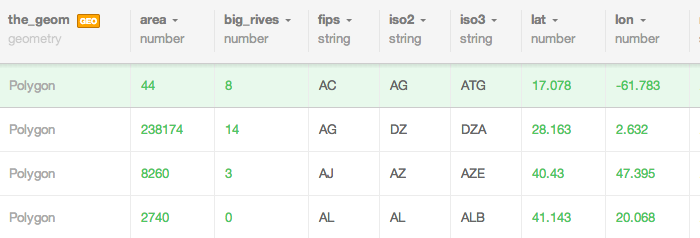
In the options, add big_rivers as the column and select Number as the type. Finally, click ‘Create column’.
Join through a SELECT statement
Now, let’s do a SELECT to see the data joined:
SELECT
  tm_world_borders_s.cartodb_id,
  COUNT(table_50m_rivers_lake_cen.cartodb_id)
FROM tm_world_borders_s, table_50m_rivers_lake_cen
WHERE ST_Intersects(
  tm_world_borders_s.the_geom,
  table_50m_rivers_lake_cen.the_geom)
GROUP BY tm_world_borders_s.cartodb_id
In the above query, we are counting all the rivers that intersect a country. Be sure that your world borders table is named tm_world_borders_s. We GROUP BY the country name so that as a result we get country name and a count of big rivers. Great!
Updating a table using a JOIN
Now lets run a similar query, but write the numeric value to the column we created earlier, big_rivers. Run the following:
UPDATE tm_world_borders_s wb
SET big_rivers = (
  SELECT COUNT(table_50m_rivers_lake_cen.cartodb_id)
  FROM table_50m_rivers_lake_cen
  WHERE ST_Intersects(
    wb.the_geom,
    table_50m_rivers_lake_cen.the_geom
  ))
In the above query, we are running the UPDATE to our new column big_rivers, but running a nested query that selects the count of all rivers that intersect it. Like the above examples, we use an alias for the name of our world borders table name, wb. You can see that the alias is then used when we run the ST_Intersects function, indicating that for every row in the wb table, we count the rivers that intersect the country geometry. We can check now the column shows the number of rivers that each country intersects with:
Mapping the results
Now, go back to the Map View for your world borders table. Click the Style option on the right hand side of your map. In the sidebar that slides out, click the overview image of the Choropleth map. In the menu, for Column select big_rivers and customize the look & feel of the map.
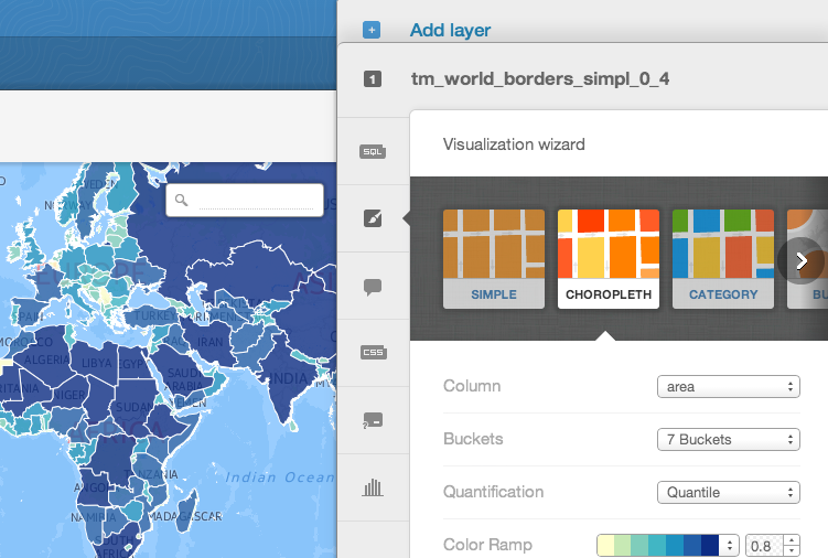
Now take a look at the map and you can see which countries the most rivers in our dataset pass through.