Spatial SQL - Part 1

In this section you’ll have the chance to test some of the most common PostGIS SQL procedures.

Set up

For this workshop, we will use CARTO as a convenient way to interact with PostGIS, which will require no installation or configuration by you. You won’t even need an account; we’re using public demo datasets.

As a client for this workshop, we will use a web application that can interact with CARTO: Franchise. You can access to an instance of it, with the CARTO connector enabled, here: https://franchise.carto.io/.

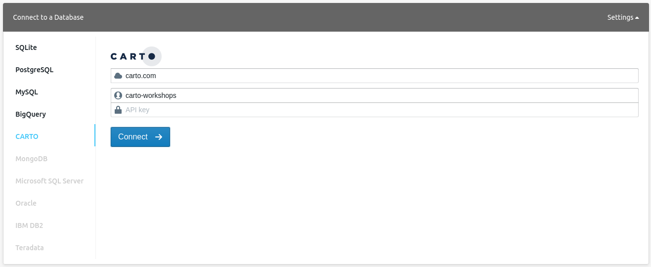
From the side menu, navigate to ‘CARTO’, then use the following parameters to connect:

• Host name: carto.com
• User name: carto-workshops
• API key: you can leave this empty

Once connected, you can run SELECT queries against any public dataset from that account.

Some tables you have available to you from this account are:

• ne_10m_populated_places_simple: Natural Earth populated places
• ne_110m_admin_0_countries: Natural Earth country boundaries
• railroad_data: Railroad accidents in the USA
• barcelona_building_footprints: Barcelona blocks
• lineas_madrid: Madrid metro lines
• listings_madrid: Madrid Airbnb listings

Try entering a simple query like the one below. To run the query, type Control+Enter on PCs, Command+Enter/Cmd+Return on macs, or press the green play button in the bottom right corner of the SQL panel.

select *
  from listings_madrid
where bathrooms >= 3

The results of your query will be displayed in a typical table view, which will allow you to explore all returned fields and rows.

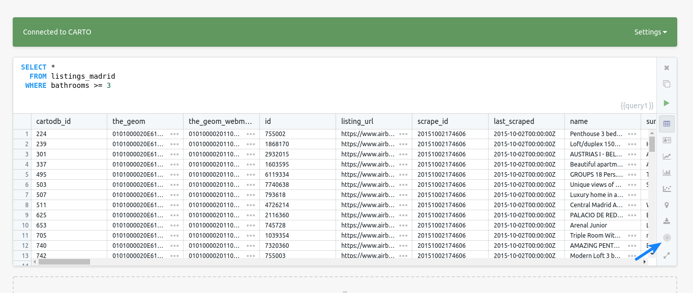
If you hit the small CARTO icon in the bottom right of the result panel, Franchise switches to a geographical result.

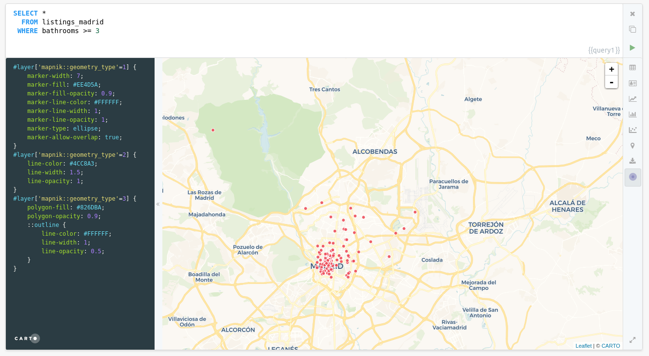
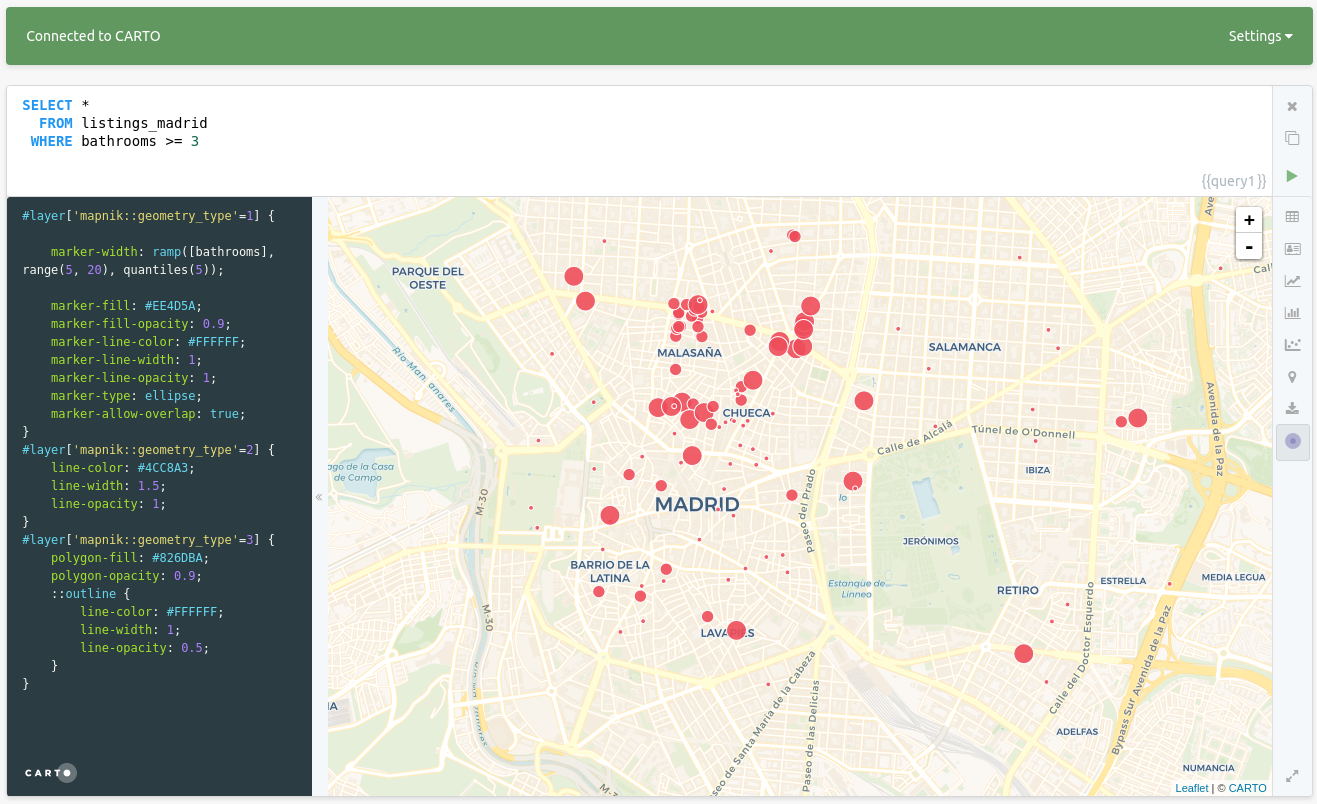
This map uses the CartoCSS language to define how data is rendered. By default, all three geometry types (points, lines, polygons) are rendered with default symbology, defined in the panel to the left. You can, however, alter the cartoCSS at any point. After making your edits, apply them by typing Control+Enter or Cmd+Enter. You can even leverage TurboCARTO to generate style ramps quickly. For example, if we wanted to style our points’ size by the number of bathrooms at each point, we can change the default marker-width from this:

 marker-width: 7;

to this:

 marker-width: ramp([bathrooms], range(5, 20), quantiles(5));

Both CartoCSS and TurboCARTO are out of the scope of this training, but you can find more training materials on the cartography section of this repository.

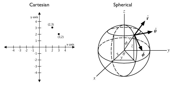
PostGIS concepts: geometry vs. geography

• Geometry uses a cartesian plane to measure and store features (CRS units):

  The basis for the PostGIS geometry type is a plane. The shortest path between two points on the plane is a straight line. That means calculations on geometries (areas, distances, lengths, intersections, etc) can be calculated using cartesian mathematics and straight line vectors.

• Geography uses a sphere to measure and store features (Meters):

  The basis for the PostGIS geography type is a sphere. The shortest path between two points on the sphere is a great circle arc. That means that calculations on geographies (areas, distances, lengths, intersections, etc) must be calculated on the sphere, using more complicated mathematics. For more accurate measurements, the calculations must take the actual spheroidal shape of the world into account, and the mathematics becomes very complicated indeed.

More about the geography type can be found here and here.

Source: Boundless Postgis intro

the_geom vs. the_geom_webmercator

• the_geom EPSG:4326. Unprojected coordinates in decimal degrees (Lon/Lat). WGS84 Spheroid.
• the_geom_webmercator EPSG:3857. UTM projected coordinates in meters. This is a conventional Coordinate Reference System, widely accepted as a ‘de facto’ standard in webmapping.

In CARTO, the_geom_webmercator column is the one we see represented in the map. Know more about projections:

• In this tutorial.
• Map Projections in Wikipedia.
• In this CARTO blog post.

Finally, remember that Builder needs the following columns to work correctly:

• cartodb_id: it has to be a column with unique values
• the_geom: is a geometry in EPSG:4326 coordinate system
• the_geom_webmercator: is a geometry field in EPSG:3857

SQL that applies to all geometries

The following queries will work on all geometries: point, line, and polygon.

Transforming geometries into a different projection

World Robinson

SELECT
  cartodb_id,
  ST_Transform(the_geom, 54030) AS the_geom_webmercator
FROM
  ne_50m_land

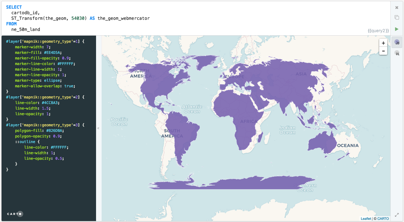
About working with different projections in CARTO and ST_Transform.

This application displays several popular map projections and gives some information on each.

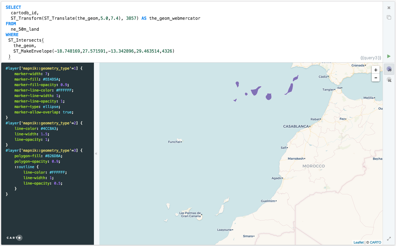
Translating Geometries

SELECT
  cartodb_id,
  ST_Transform(ST_Translate(the_geom,5.0,7.4), 3857) as the_geom_webmercator
FROM
  ne_50m_land
WHERE
 ST_Intersects(
   the_geom,
   ST_MakeEnvelope(-18.748169,27.571591,-13.342896,29.463514,4326)
 )

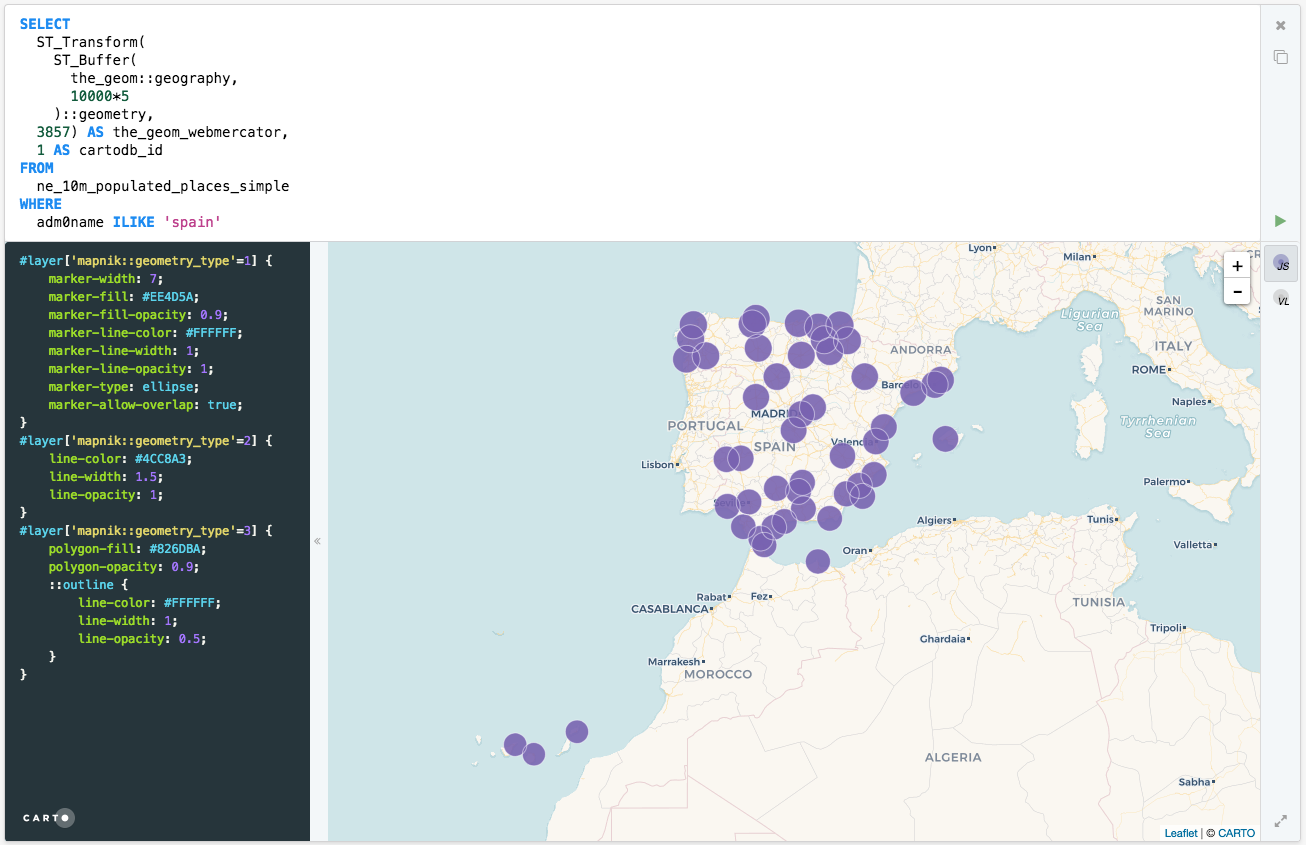
Buffer (ST_Buffer)

Simple Buffer

ST_Buffer uses the input geometry’s unit of measure, which in the case of our the_geom is decimal degrees. In order to use meters as our buffer unit, we must cast our geometry to a geography, then back to a geometry once we have our buffer. Alternatively, if you just want to visualize you can simply use the_geom_webmercator, as it’s unit of measure is already meters.

About ST_Buffer.

SELECT
  ST_Transform(
    ST_Buffer(
      the_geom::geography,
      10000*5
    )::geometry,
  3857) As the_geom_webmercator,
  1 as cartodb_id
FROM
  ne_10m_populated_places_simple
WHERE
  adm0name ILIKE 'spain'

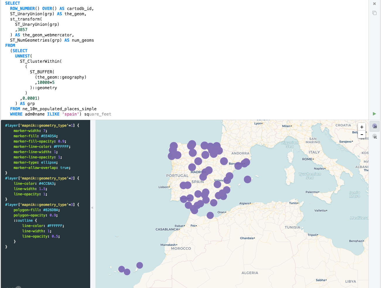
Dissolve Buffers

SELECT
  row_number() over() as cartodb_id,
  ST_UnaryUnion(grp) as the_geom,
  st_transform(
    ST_UnaryUnion(grp)
    ,3857
  ) as the_geom_webmercator,
  ST_NumGeometries(grp) as num_geoms
FROM
  (SELECT
    UNNEST(
      ST_ClusterWithin(
        (
          ST_BUFFER(
            (the_geom::geography)
            ,10000*5
          )::geometry
        )
      ,0.0001)
    ) AS grp
  FROM ne_10m_populated_places_simple
  WHERE adm0name ILIKE 'spain') sq

SQL for Points

Know wether a geometry is within the given range from another geometry:

SELECT a.*
  FROM ne_10m_populated_places_simple a,
       ne_10m_populated_places_simple b
 WHERE a.cartodb_id != b.cartodb_id
   AND ST_DWithin(
         a.the_geom_webmercator,
         b.the_geom_webmercator,
         150000)
   AND a.adm0name = 'Spain'
   AND b.adm0name = 'Spain'

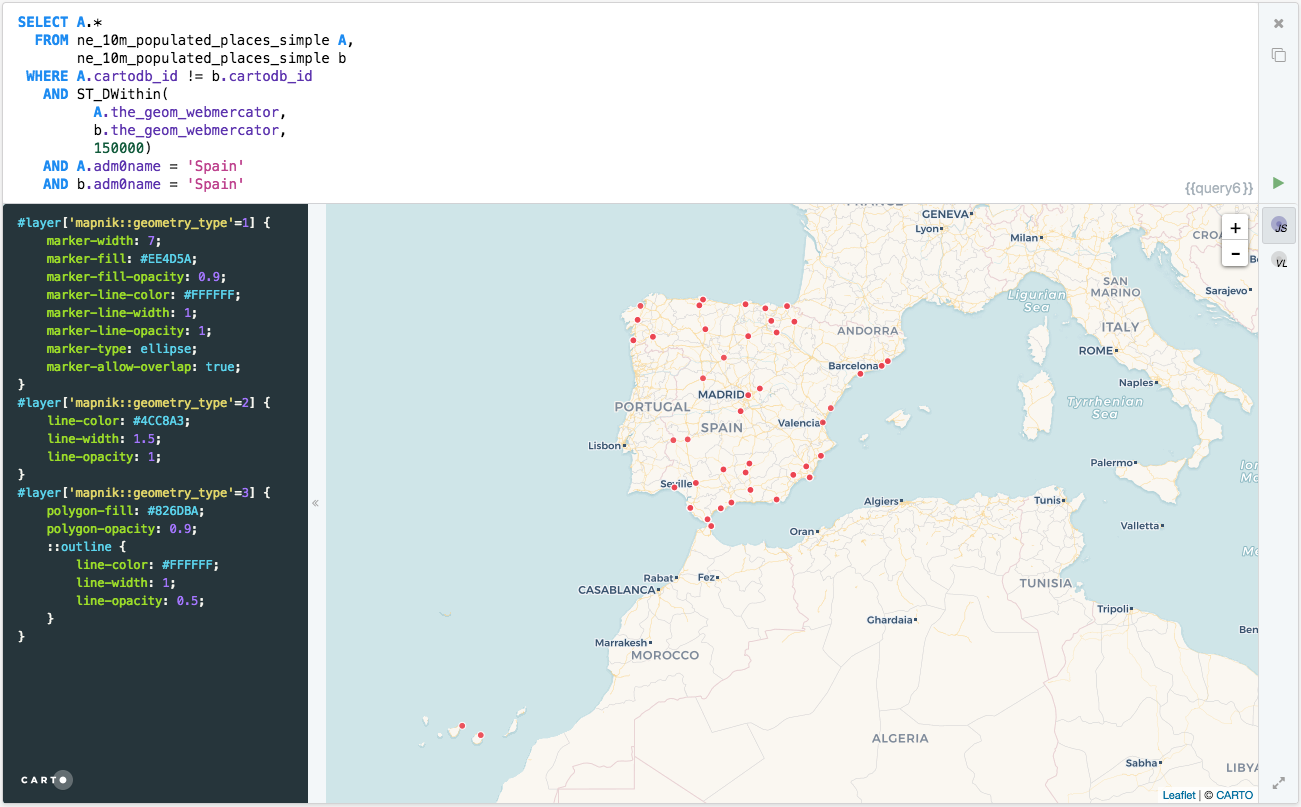
In this case, we are using the_geom_webmercator to avoid casting to geography type. Calculations made with geometry type takes the CRS units.

Keep in mind that CRS units in webmercator are not meters, and they depend directly on the latitude.

About ST_DWithin.

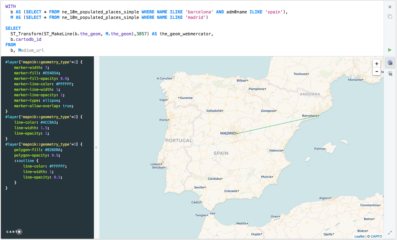
Making lines

Simple lines

WITH
  b as (SELECT * FROM ne_10m_populated_places_simple WHERE name ilike 'barcelona' and adm0name ilike 'spain'),
  m as (SELECT * FROM ne_10m_populated_places_simple WHERE name ilike 'madrid')

SELECT
  ST_Transform(ST_MakeLine(b.the_geom, m.the_geom),3857) as the_geom_webmercator,
  b.cartodb_id
FROM
  b, m

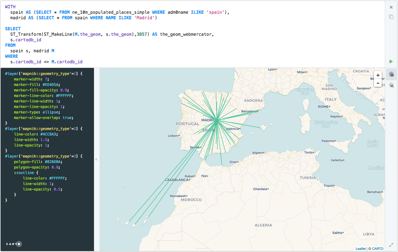
Multiple lines

WITH
  spain as (SELECT * FROM ne_10m_populated_places_simple WHERE adm0name ILIKE 'spain'),
  madrid as (SELECT * FROM spain WHERE name ILIKE 'Madrid')

SELECT
  ST_Transform(ST_MakeLine(m.the_geom, s.the_geom),3857) as the_geom_webmercator,
  s.cartodb_id
FROM
  spain s, madrid m
WHERE
  s.cartodb_id <> m.cartodb_id

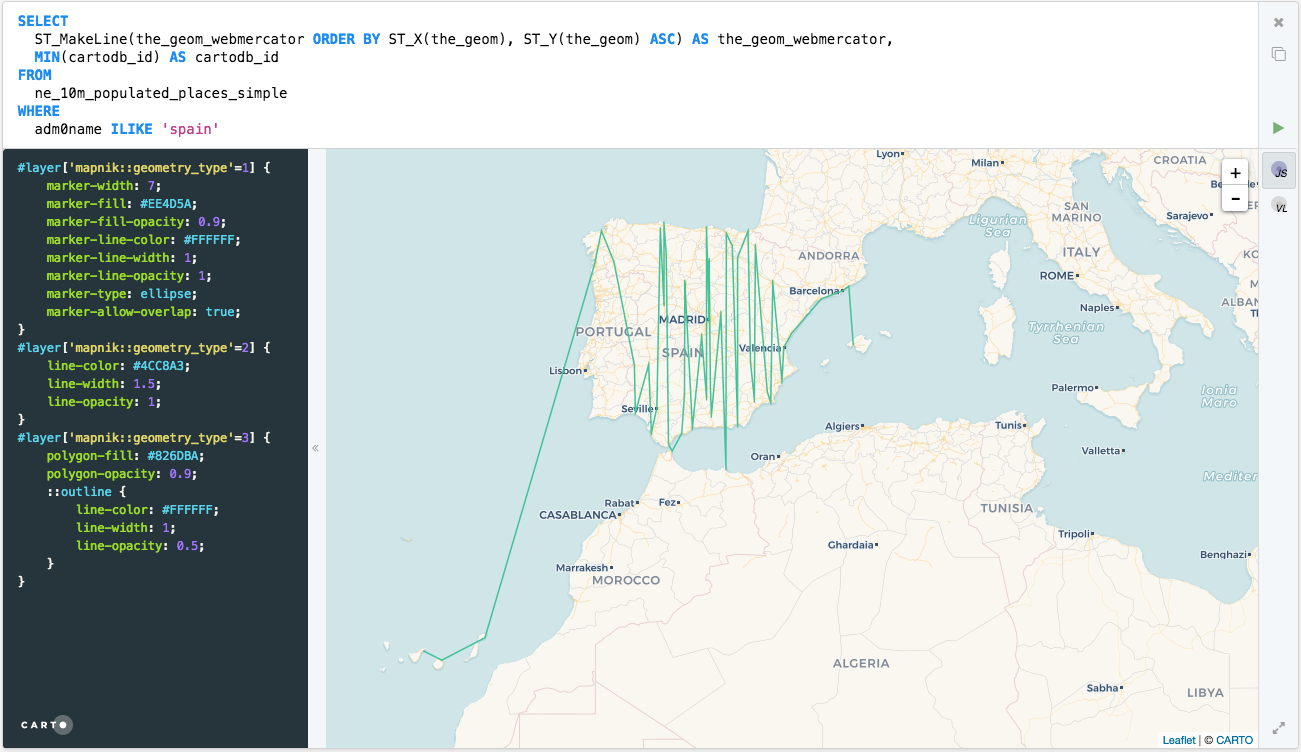
Sequential lines

SELECT
  ST_MakeLine(the_geom_webmercator ORDER BY ST_X(the_geom), ST_Y(the_geom) ASC) as the_geom_webmercator,
  min(cartodb_id) as cartodb_id
FROM
  ne_10m_populated_places_simple
WHERE
  adm0name ILIKE 'spain'

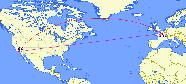
Great Circles (curved lines)

 SELECT ST_Transform(
          ST_Segmentize(
            ST_Makeline(
              a.the_geom,
              b.the_geom
            )::geography,
            100000
          )::geometry,
        3857
        ) as the_geom_webmercator
   FROM (
          SELECT *
            FROM ne_10m_populated_places_simple
           WHERE name ILIKE 'madrid'
        ) as a,
        (
          SELECT *
            FROM ne_10m_populated_places_simple
           WHERE name ILIKE 'new york'
        ) as b

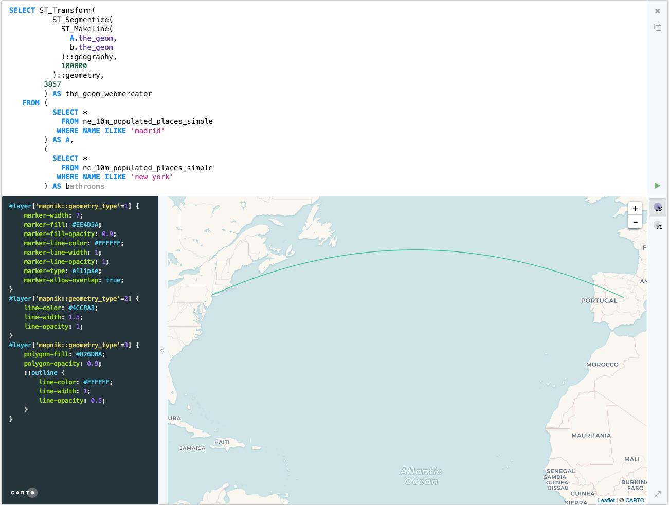
About Great Circles.

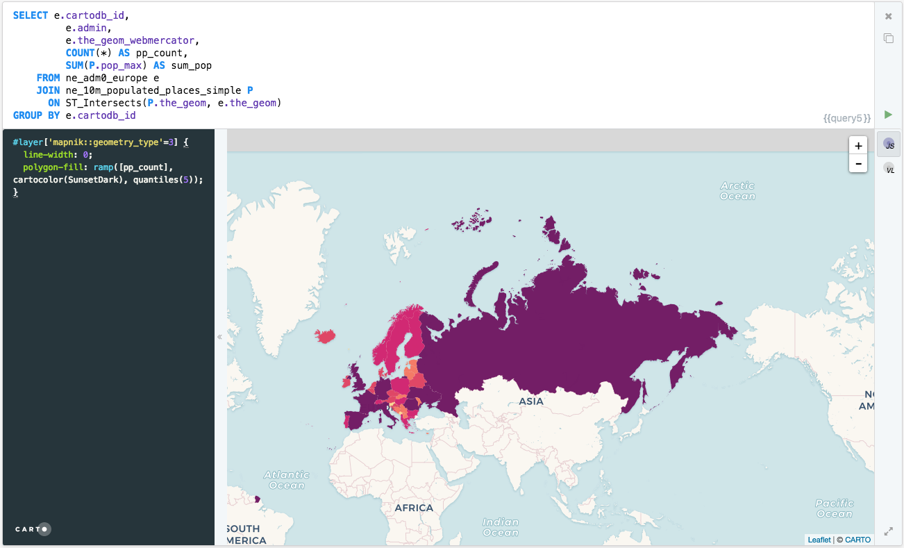
SQL for Polygons

Get the number of points inside a polygon

Using GROUP BY:

  SELECT e.cartodb_id,
         e.admin,
         e.the_geom_webmercator,
         count(*) AS pp_count,
         sum(p.pop_max) as sum_pop
    FROM ne_adm0_europe e
    JOIN ne_10m_populated_places_simple p
      ON ST_Intersects(p.the_geom, e.the_geom)
GROUP BY e.cartodb_id

Using LATERAL:

SELECT a.cartodb_id,
       a.admin AS name,
       a.the_geom_webmercator,
       counts.number_cities AS pp_count,
       counts.sum_pop
  FROM ne_adm0_europe a
 CROSS JOIN LATERAL
  ( SELECT count(*) as number_cities,
           sum(pop_max) as sum_pop
      FROM ne_10m_populated_places_simple b
     WHERE ST_Intersects(a.the_geom, b.the_geom)
  ) AS counts

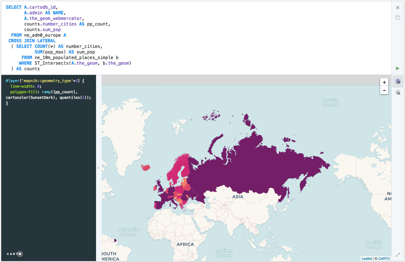
About ST_Intersects and Lateral JOIN

Note: You know about the EXPLAIN ANALYZE function? use it to take a look on how both queries are pretty similar in terms of performance.

Get the difference between two geometries:

SELECT a.cartodb_id,
       ST_Difference(
         a.the_geom_webmercator,
         b.the_geom_webmercator
       ) AS the_geom_webmercator
  FROM ne_50m_land a,
       ne_adm0_europe b
 WHERE b.adm0_a3 like 'ESP'

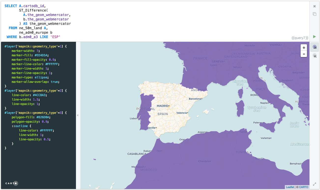
About ST_Difference.

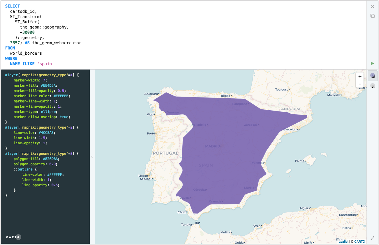
Negative buffer

SELECT
  cartodb_id,
  ST_Transform(
    ST_Buffer(
      the_geom::geography,
      -30000
    )::geometry,
  3857) As the_geom_webmercator
FROM
  world_borders
WHERE
  name ilike 'spain'

Spatial Joins

with metro_lines as (
  SELECT
    row_number() over() as cartodb_id,
    ST_Buffer(
        the_geom::geography,
        100
      )::geometry as the_geom,
    ST_Transform(
      ST_Buffer(
        the_geom::geography,
        100
      )::geometry,
    3857) As the_geom_webmercator
  FROM lineas_madrid
  )

select x.*,
y.cartodb_id as joined
from listings_madrid x
left join metro_lines y
on st_intersects(x.the_geom, y.the_geom)

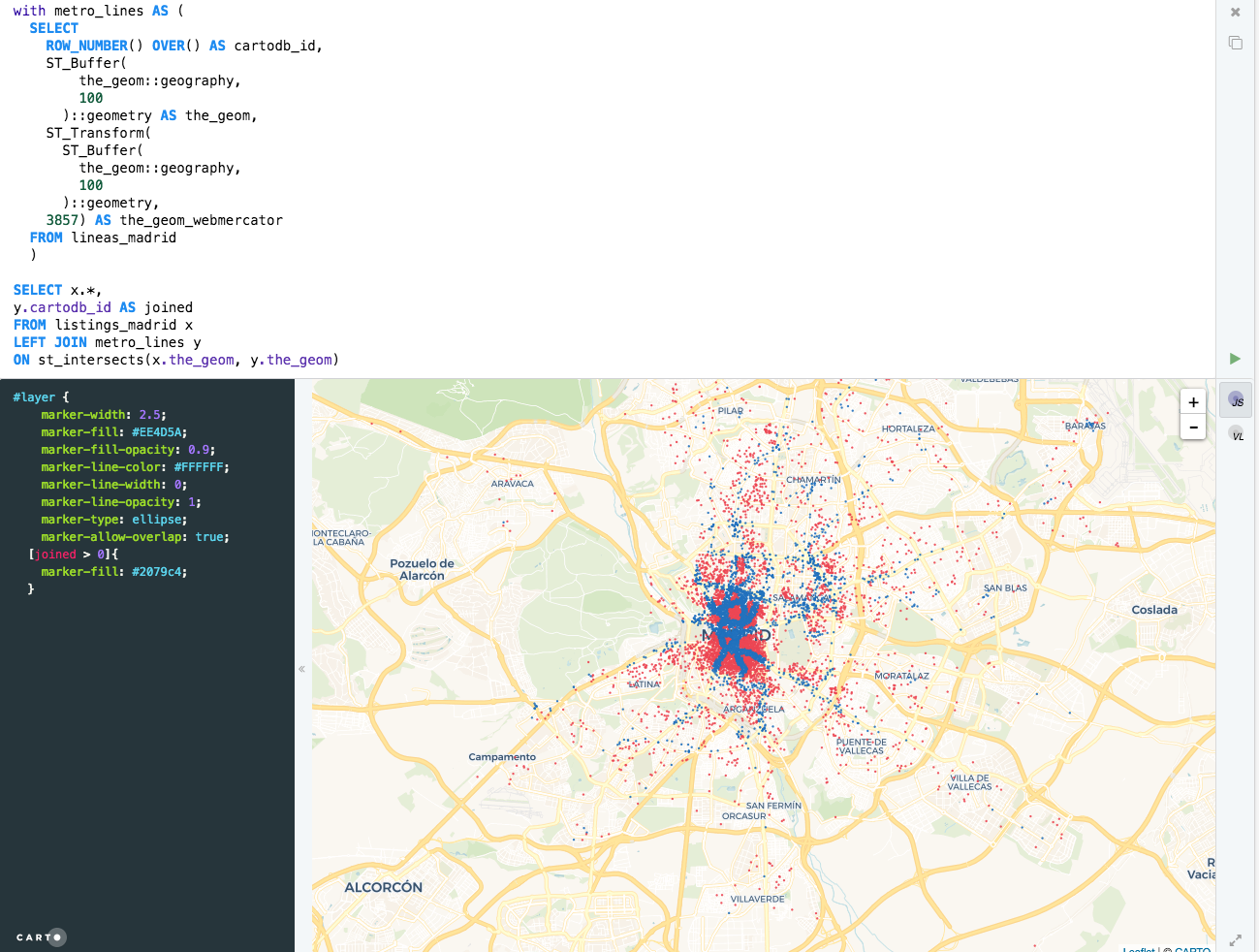
In the above example, you can see where the points joined on the buffer of the metro lines, and where they didn’t based on if the cartodb_id for the lines existed in the points dataset.

SQL for CARTO

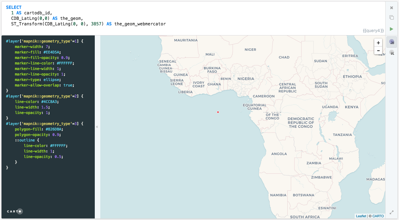
CDB_LatLng()

cdb_latlng() is a shortcut to the function ST_SetSRID(ST_Point(),srid), with the default srid set as 4326, the srid of the_geom. One notable difference is that ST_Point() takes coordinate pairs in the order of (longitude, latitude), whereas cdb_latlng() takes coordinate pairs in the order of (latitude, longitude).

SELECT
  1 as cartodb_id,
  CDB_LatLng(0,0) as the_geom,
  ST_Transform(CDB_LatLng(0, 0), 3857) as the_geom_webmercator
  /* ST_SetSRID(ST_MakePoint(0, 0), 4326) */

Grids

Hexagon Grids

WITH grid as (
  SELECT
    row_number() over () as cartodb_id,
    CDB_HexagonGrid(
      ST_Buffer(the_geom_webmercator, 1000000),
      10000
    ) AS the_geom_webmercator
  FROM
    world_borders
  WHERE
    name ILIKE 'spain')

SELECT
  grid.the_geom_webmercator,
  grid.cartodb_id
FROM
  grid, world_borders a
WHERE
  ST_Intersects(grid.the_geom_webmercator, a.the_geom_webmercator)
AND
  name ILIKE 'spain'

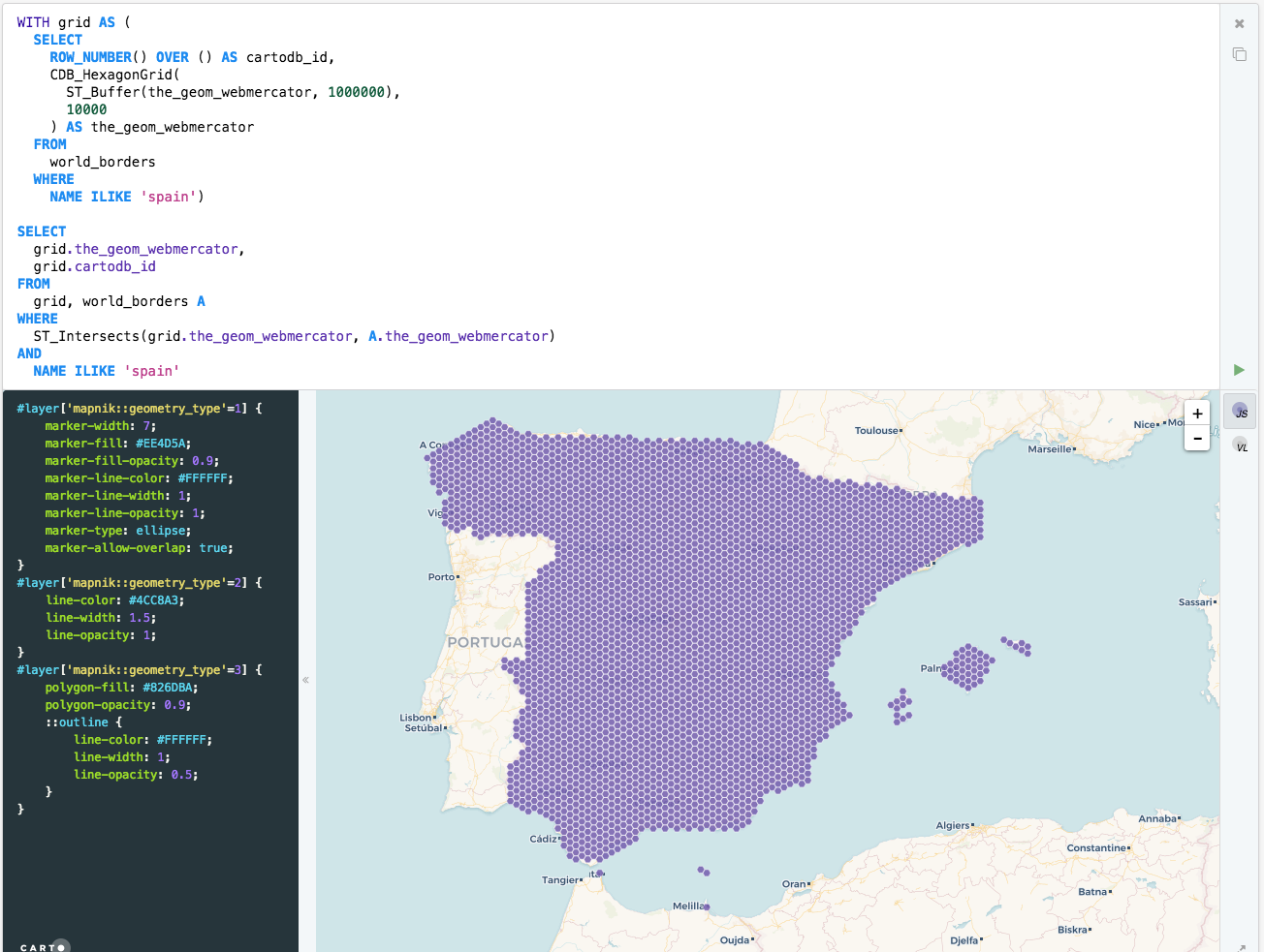
About CDB_HexagonGrid

Rectangular Grids

WITH grid as (
  SELECT
    row_number() over () as cartodb_id,
    CDB_RectangleGrid(
      ST_Buffer(the_geom_webmercator, 1000000),
      25000,
      25000
    ) AS the_geom_webmercator
  FROM
    world_borders
  WHERE
    name ILIKE 'spain')

SELECT
  grid.the_geom_webmercator,
  grid.cartodb_id
FROM
  grid, world_borders a
WHERE
  ST_Intersects(grid.the_geom_webmercator, a.the_geom_webmercator)
AND
  name ILIKE 'spain'

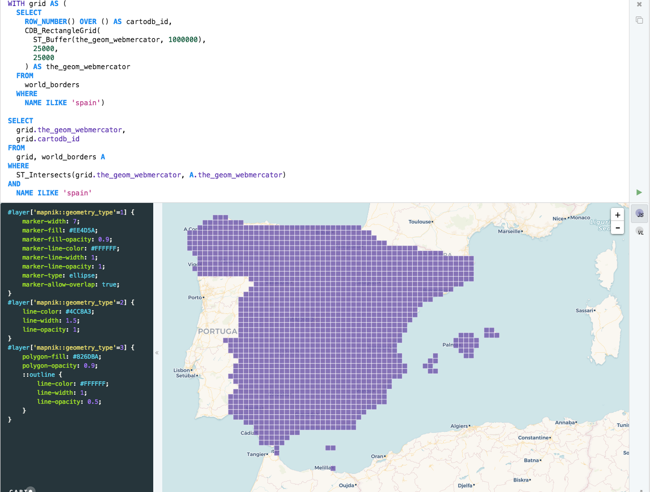
About CDB_RectangleGrid

You can read more about CARTO custom spatial queries here.