Geoprocessing with PostGIS - Part 1

CartoDB is built on top of PostGIS  the powerful add-on that turns PostgreSQL into a spatial database.  Many popular Geoprocessing functions in GIS software can be done with PostGIS queries  and this blog series will provide a one-for-one replication of the functions in QGIS' Vector>Geoprocessing Tools menu.

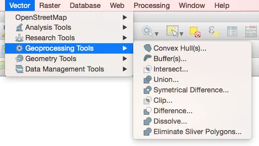
In QGIS  the Vector menu has all sorts of goodies  but we'll focus on the Geoprocessing Tools submenu  which has Convex Hulls  Buffers  Intersects  Unions  Dissolves  and more.  If you're making maps  these are important tools for the data-munging process  and with a little SQL and PostGIS you can do them right here in CartoDB!  We'll start with two:  Convex Hull and Buffer.

Convex Hull

A Convex Hull is the smallest convex polygon that can contain a set of other geometries. The process is often described as stretching out a rubber band around a set of points  which will constrict to its smallest possible shape. Why would you use a convex hull in mapping?  There are a few use cases: They can be useful for highlighting patterns in data and visualizing coverage areas.  This whitepaper from Azavea uses them to analyze the "compactness" of congressional districts.  

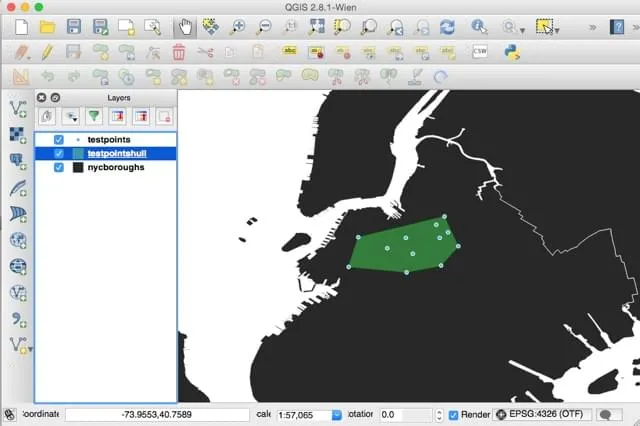
Let's start with a set of 12 random points over Brooklyn. With the points loaded in QGIS (with a nice borough boundary layer courtesy of the New York City Planning Department)  running the Convex Hull wizard will generate a new shapefile with a single polygon that encompasses all 12 points.  Here's what the new convex hull looks like on the map:

Now let's load the same data into CartoDB and name its table testpoints.  

PostGIS has a function called ST_ConvexHull() that will generate a convex hull from a collection of geometries.  However  our testpoints dataset is a bunch of individual points  so we must first collect them into a geometry collection using ST_Collect().  

So  our first pass at at a convex hull SQL statement looks like:

##_INIT_REPLACE_ME_PRE_##
SELECT ST_ConvexHull(
 ST_Collect(
   the_geom
 )
) AS the_geom
FROM testpoints
##_END_REPLACE_ME_PRE_##

This will work  but remember that we must have a the_geom_webmercator field in our result set for CartoDB to render it on the map.  To accomplish this  we use ST_Transform() to convert the WGS84 coordinates in the_geom to web mercator coordinates for mapping:

##_INIT_REPLACE_ME_PRE_##
SELECT ST_ConvexHull(
 ST_Collect(
   the_geom
 )
) AS the_geom
ST_Transform(
 ST_ConvexHull(
   ST_Collect(
     the_geom
   )
 )
 3857
) AS the_geom_webmercator
FROM testpoints
##_END_REPLACE_ME_PRE_##

There's our Convex Hull!  This isn't very useful on its own  but you could use this new polygon in combination with others in your analysis  or save it as a new table using Dataset from Query in the CartoDB Edit menu.

Buffer

A buffer is simply a polygon whose border is a specified distance from another geometry or group of geometries.  The resulting polygon can be used as a visual element on the map  or can be used for further spatial queries (this is not optimal  but that's another blog post.  Check out how Andy uses it in this academy lesson on finding blues musician birthplaces within the Buffer).

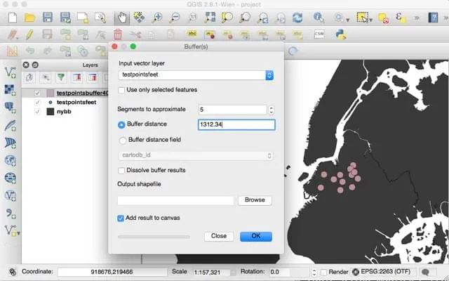
Let's see about the creation of buffers in QGIS.  In the screenshot below  you'll see a buffer running on testpointsfeet.  This is our original testpoints dataset converted from WGS84 to NY State Plane  as Buffer will always use the units of the selected layer's coordinate reference system.  Buffers in degrees wouldn't be very useful  so switching to NY State Plane (EPSG:2266) allows us to run the buffer in feet. (1312.24 feet = 400 meters)  We can see the new polygon layer is a series of circles around the original points.  If these were real features  such as Restaurants or Dry Cleaners in an area  we can imagine the new buffers showing us their 5-minute delivery areas.

There's also a handy checkbox in the wizard that allow us to dissolve the resulting buffers into a single feature.  Let's see what this looks like:

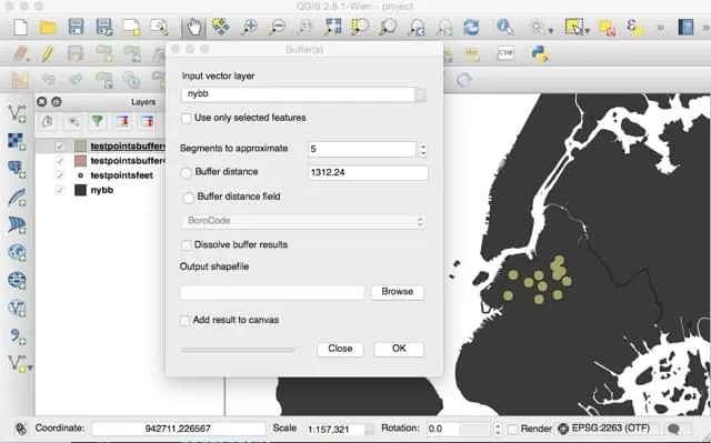
Where the original buffers were overlapping  we now see them consolidated into a single polygon.  

Now let's run the same buffer in CartoDB using ST_Buffer().  The docs tell us that there are 4 ways we can call ST_Buffer()  3 of which are expecting a geometry  type plus the units for the buffer  and one which expects a geography type plus meters.  (More on geography vs geometry here.)    CartoDB's the_geom column is a geometry  so we can recast it as geography using ::geography as it is passed to ST_Buffer()  then recast the results back to ::geometry for mapping.  So  our first pass at a 400m Buffer query looks like this:

##_INIT_REPLACE_ME_PRE_##
SELECT ST_BUFFER(
 the_geom::geography
 400
)::geometry as the_geom
FROM chriswhong.testpoints
##_END_REPLACE_ME_PRE_##

Just like before  we have to include the_geom_webmercator for CartoDB to map the results  and that requires using ST_Transform() again:

To dissolve the results just like we did in QGIS  we'll use the ST_Union() PostGIS function:

Here's an example of buffers used in a finished map  showing 5 and 10-minute walking circles around Boston's Subway Stations.

Thanks for reading!  In the next installment  we'll cover the PostGIS equivalent of Intersect and Union.  Stay tuned to learn how the power of PostGIS can make your maps shine.

Happy Mapping!!