3 ways to load geospatial data into Redshift

Update March 15th, 2023: Now you can import geospatial data to Amazon Redshift using CARTO!

Amazon Redshift has multiple ways to load data both native COPY commands and through other tools. With that said, loading geospatial data always has added complexity. If your data is not in a CSV format or has things like misformatted geometries, you will have to take a few extra steps to load your data.

This post outlines four ways to load your geospatial data into Redshift, and some tools and methods you can use along the way.

We covered this guide because importing geospatial data into Amazon Redshift came with challenges. And it became clear we could integrate a solution into our platform.

Following our product announcement, these are the steps you will follow in CARTO:

• Go to your CARTO Workspace, 
• Create a Redshift connection in “Connections”
• Check your Redshift data in “Data Explorer” and click on “Import data”
• Start importing files using our Import UI, from your computer or from a URL.

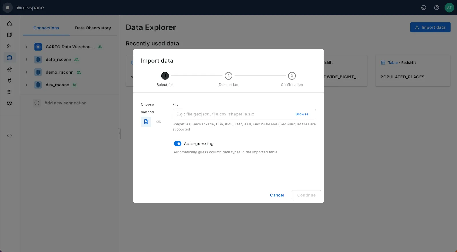
And that’s it! Your geospatial data will instantly be imported to Amazon Redshift, and using CARTO you’ll even be able to quickly preview it.

You can find more detailed instructions, plus all the available formats in our Documentation. Additionally, you will be able to use our Import API to import files programmatically.

Want to have a go yourself? Sign up to a free CARTO two-week trial.

Option 1: Load your data with Python

This post from our own Borja Muñoz outlines a step by step approach to transforming the data, loading the data to S3, and then using the Redshift Data API and the boto3 Python package to load your data. The process uses the following steps:

1. Create a CSV file with EWKB geometries using Fiona and Shapely
2. Upload that data to S3 using boto
3. Import the data into Redshift using the Redshift Data API
4. The code includes a function to read the data types from Fiona and create the table which is required to execute the COPY command.

You can check out the full post here and get access to the code here.

Option 2: Load with the CSV COPY command

This process is very similar to the Python route but using the native tools within AWS. The process will:

1. Transform your geospatial data to a CSV using GDAL
2. Upload the data to S3
3. Generate a CREATE TABLE statement using the ddl-generator command line tool
4. Run the COPY command in Redshift

For this tutorial we are going to load in 311 data from Los Angeles. You can download the data here. Just hit export and CSV.

Transform your geospatial data to a CSV using GDAL

First you need to install GDAL if you don’t have it. Here is a guide to do so with Homebrew on a Mac and on Windows.

For this step we can create a geometry on our CSV file in GeoJSON from the latitude and longitude columns. To do so you can run this command in the file location on your computer:

ogr2ogr -f csv -dialect sqlite -sql "select AsGeoJSON(MakePoint(Longitude, Latitude)) AS geom, * from la_311" la_311_new.csv la_311.csv

Note: I renamed my file to la_311.csv to save on keystrokes.

You can do this for any file type supported by GDAL including Shapefiles, GeoJSON, KML, Geoparquet, and more.

Upload the data to S3

Next we can upload our data to AWS S3. We can use the AWS Console or by using the AWS command line tools. If you need help setting this up you can use this guide from the AWS S3 documentation.

  aws s3 cp la_311_new.csv s3://mybucket

Once that is finished your table will be in S3.

Generate a CREATE TABLE statement using the ddl-generator command line tool

Before you can copy your table, you need to create the table in Redshift using a CREATE TABLE command. You can manually create this  otherwise you can use a Python script or the ddl-generator library to do so on the command line. I used the last option and this builds a SQL file to run in Redshift.

  ddlgenerator postgresql la_311_new.csv > la_311_new.sql

Which returns this SQL:

 CREATE TABLE la_311 (
    srnumber VARCHAR(12) NOT NULL,
    createddate TIMESTAMP WITHOUT TIME ZONE NOT NULL,
    updateddate TIMESTAMP WITHOUT TIME ZONE NOT NULL,
    actiontaken VARCHAR(24) NOT NULL,
    owner VARCHAR(5),
    requesttype VARCHAR(26) NOT NULL,
    status VARCHAR(12) NOT NULL,
    requestsource VARCHAR(29) NOT NULL,
    mobileos VARCHAR(7),
    anonymous BOOLEAN NOT NULL,
    assignto VARCHAR(17),
    servicedate TIMESTAMP WITHOUT TIME ZONE,
    closeddate TIMESTAMP WITHOUT TIME ZONE,
    addressverified VARCHAR(1) NOT NULL,
    approximateaddress BOOLEAN,
    address VARCHAR(70),
    housenumber INTEGER,
    direction VARCHAR(5),
    streetname VARCHAR(29),
    suffix VARCHAR(5),
    zipcode VARCHAR(5),
    latitude DECIMAL(14, 12),
    longitude DECIMAL(15, 12),
    location VARCHAR(36),
    tbmpage INTEGER,
    tbmcolumn VARCHAR(1),
    tbmrow INTEGER,
    apc VARCHAR(21),
    cd INTEGER,
    cdmember VARCHAR(23),
    nc INTEGER,
    ncname VARCHAR(96),
    policeprecinct VARCHAR(16)
  );

Keep in mind that this will generate the file with specific values for the data types, such as VARCHAR(96). I have sometimes experienced issues with the data in the CSV not perfectly matching that schema. Just open a text editor and remove the parentheses and number (“VARCHAR(96)” to “VARCHAR”) and that should fix the issue.

Run the COPY command in Redshift

Finally just run the copy command in Redshift to fill your table with data from the CSV. The command will look like this.

 copy la_311
  from 's3://mybucket/la_311.csv'
  iam_role 'arn:aws:iam::<aws-account-id>:role/<role-name>';

There are lots of options and parameters so make sure to check the documentation out to find all those options.

Option 3: Use Airbyte and dbt

One of my favorite tools I have come across recently is Airbyte. It is an ELT tool (Extract  Load  Transform). You can install the open source version of Airbyte using docker in a few simple steps. That will install the system and allow you to access their user interface. From here you can create sources  destinations  and connections.

This makes the ingestion process easier  especially if you have data that is regularly updated with the same data structure  or if you have transformations you want to continually run on your data.

Install Airbyte

The first step is to install Airbyte. This is a simple process if you have Docker up and running. You can find the instructions here and you should be ready in a few minutes. You can install it in three steps locally with Docker or in AWS.

Create CSV Source

The next step is to create a CSV source. The best way to do this is to host your file in S3 and connect it to Airbyte once it has been loaded. Click on Source and enter the fields.

Create Redshift Destination

Repeat the process to set up a destination in Redshift.

Create and run Connection

Next we create our connection between the two sources. Make sure to select the option to Normalize the data rather than raw JSON as this will generate the dbt project.

Airbyte is an ELT tool  which focuses on extracting and loading the data as raw JSON  then leveraging the destination to do the transformations at scale  which Redshift is perfectly suited for using its scalable compute processing. When we normalize the data, we generate the dbt files which allow us to customize that step.

Build and extract dbt project files

Once the sync has run you can generate and run the dbt project and files within Airbyte. This will also allow you to export the files to upload to AWS and modify. Follow these instructions from the documentation to generate the SQL files and then export the dbt files (here is a guide to exporting the desired files from EC2 to S3).

Set up dbt in AWS Cloud9 and deploy model

Next I am going to create a new AWS Cloud9 instance, a virtual IDE that will allow me to run everything inside AWS using my credentials, and upload the dbt project files I exported from Airbyte. Below are the steps to set up and run the project (note: I had to make some changes to file locations and this may vary based on your setup).

Run the dbt debug statement

dbt debug --profiles-dir /home/ec2-user/environment/normalize

Install dbt dependencies

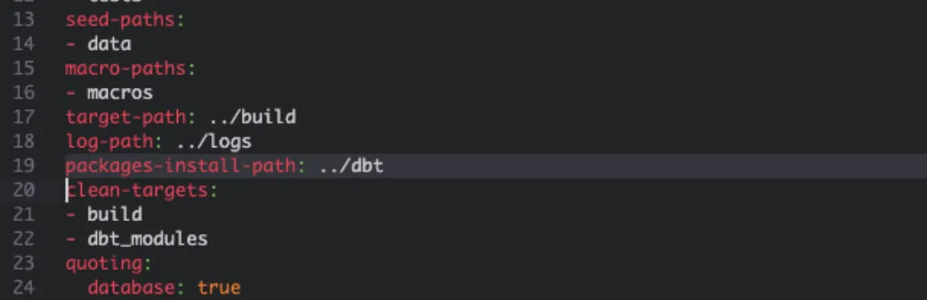
Modify the dbt_project.yml file to set a new dependencies location at packages-install-path:

Then run:

dbt deps --profiles-dir /home/ec2-user/environment/normalize

Modify the SQL file to create a geometry

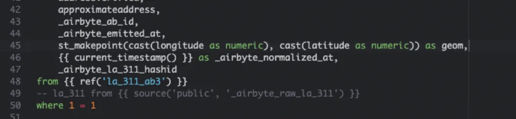
Let’s start with a simple transformation to create a geometry in our table. Open the SQL file located at ../models/airbyte_tables/public/la_311.sql. You should see the dbt generated SQL here. We are going to modify one line to create a geometry from the latitude and longitude columns. We need to cast the values to numeric within the ST_MakePoint function.

 st_makepoint(cast(longitude as numeric), cast(latitude as numeric)) as geom

Of course  you can modify any part of this statement to adjust the data or add new columns. For repeatable data ingestion this is extremely valuable as you can write this code once and then run the pipeline as needed.

Run the new pipeline

Once you have saved your files  you can now run the new pipeline:

  dbt run --profiles-dir /home/ec2-user/environment/normalize

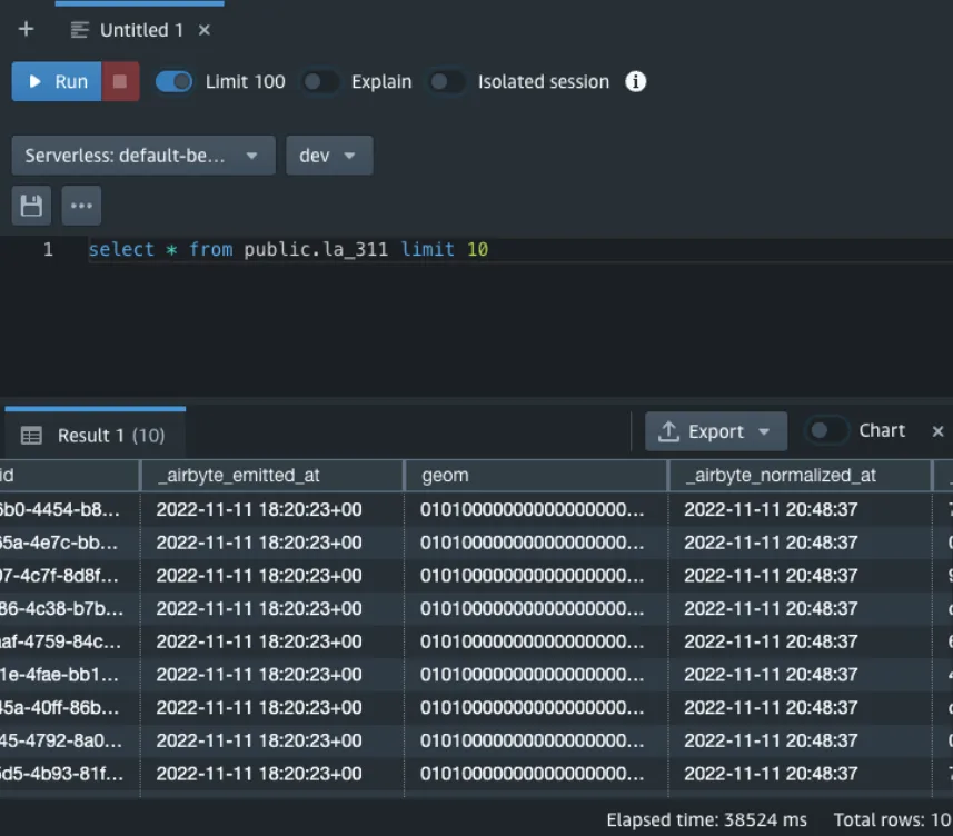
Once this completes you should see your new column in your table in Redshift.

If you want to automate this you can load the dbt project to GitHub and link it to the Airbyte by following this guide.

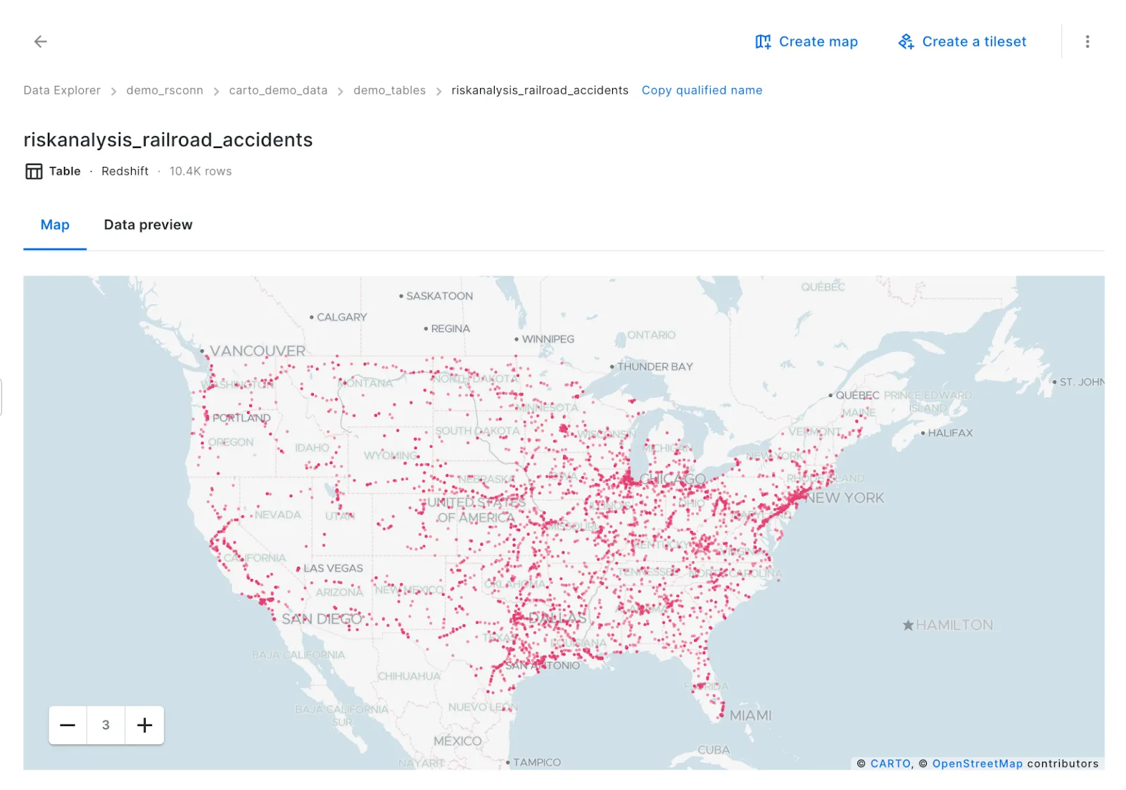
Once your data is loaded and Redshift is connected to CARTO, you can start visualizing your data in Builder and running analysis using the CARTO Analytics Toolbox for Redshift.

The Los Angeles 311 data loaded in a CARTO map.

Open this in full screen here (recommended for mobile users).

Access the ultimate guide to navigating the new geospatial landscape. Download the free report: Modernizing the Geospatial Analysis Stack today.

Want to get started?

Sign up for a free 14-day trial