Building a Recommendation System for Site Planning

When it comes to Site Planning applications  organizations have a strong desire to combine data from different sources not only to derive insights at a particular location but also to compare different geographic locations (for example to find locations that show similar characteristics).

If our aim is to compare two geographic locations  we may want to take into account a variety of data points measured at that location  both from 'traditional' sources (e.g. the census) as well as from more modern sources such as mobile  financial transactions  and point of interest (POI) data.

Building our Similarity Score

Over the past few months on CARTO's specialist Spatial Data Science team  we have developed a method to compute a similarity score with respect to an existing site for a set of target locations  which can prove an essential tool for Site Planners looking at opening  relocating  or consolidating their site network.

Calculating a similarity score between two locations really boils down to computing for each variable of interest  the difference between its values at these locations  or as would be called in the following  the 'distance in variable space'  as opposed to geographical distance.

In order to estimate the similarity between two locations we first need to define what we mean by 'location'. For example  some data might be available at point level (e.g. POI data)  while others might already come spatially aggregated (e.g. census data is typically available at a given administrative unit level)  and different data sources might be available at different spatial resolutions. In fact  spatial aggregation may be necessary to create meaningful units for analysis or might be a bi-product of data anonymization procedures to ensure data privacy (e.g. in the case of mobile GPS data). So the question is: how do we select a common spatial resolution to define a meaningful unit for the analysis? And then how do we integrate data sources at different spatial resolutions to the chosen spatial support?

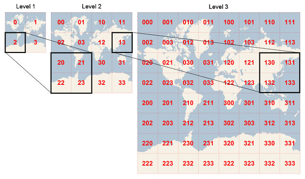
Quadkeys generation. In this example  cell 2 is the parent of cells 20 through 23  and cell 13 is the parent of cells 130 through 133. Source

This very question is what led us to develop CARTOgrid  which defines a common spatial support that can be used to integrate data available at different spatial resolutions on a regular grid where each grid cell is uniquely defined by a one-dimensional string of bits called quadtree keys  or "quadkeys" for short. The quadkeys partition the world into cells: the smaller the cells that you have  the more bits are required to address them  with the length of a quadkey corresponding to the level of zoom of the corresponding cell. Moreover  the quadkey of any cell starts with the quadkey of its parent cell (the containing cell at the previous zoom level  as seen above).

In the preliminary version of the CARTOgrid (which is used below) the integration happens by areal interpolation. Given an aggregated variable of interest at its original spatial resolution  its value on the common support defined by the CARTOgrid is obtained by averaging the values of the intersecting cells  weighted by the intersecting area. The map below shows an example of the total population from the Census interpolated on the CARTOgrid:

 View this example

An example of site selection based on similarity with a shared workspace company

Now  imagine that you have access to both third party and CARTO-curated data sets from our Data Observatory on the common support provided by the CARTOgrid  and you want to compute a similarity score between different locations using this data. For example  imagine that a market leader in the shared work space industry would like to use more data to drive their rapid expansion strategy.  

Let's imagine we want to take into account this company's sites in NYC  combining demographic  financial  and POI data stored on the CARTOgrid to find locations in LA that have similar characteristics. The results of this similarity analysis will indicate the best spots where they should plan on opening a new space/relocating an existing space with similar characteristics to the target locations in NYC.

The first step is to select the relevant variables we would like to include in our analysis. Here  we used a combination of demographic  POI  and financial data. Then  as mentioned above  the goal is to compute the (one-to-one) distance in variable space:

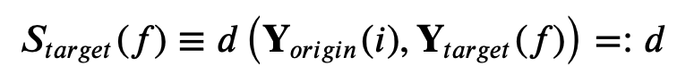
between a selected origin cell (i) and each target cell (f)  where the index j identifies the variable type (e.g. total population). For this use case  the target area here is the whole city of LA:

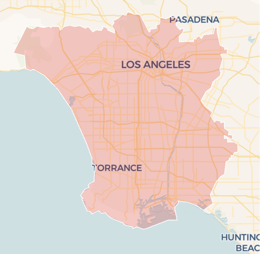
Target area for the similarity analysis

Although the method seems pretty straightforward  to properly compute distances  we need to take into account a few drawbacks.

What happens when the variables have different variances?

It is clear that in this case that distances in total population will be given a different weight than the distances in the number of food POIs:

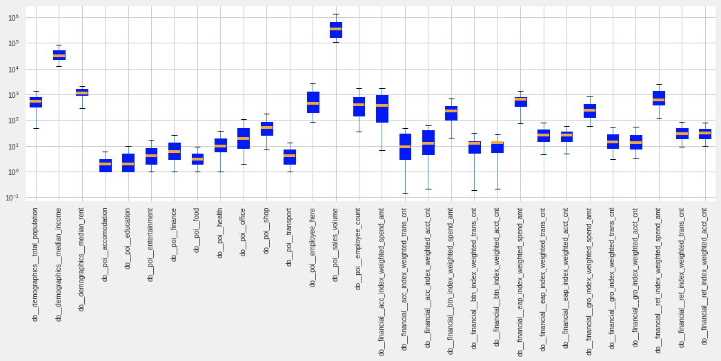
 Boxplot of the selected variables in the analysis. Note the logarithmic scale on the y-axis.

To account for different variances  the data are standardized such that they have zero mean and unit variance. This implies that all variables are given the same weight when computing distances.

What happens when there are correlations between variables?

When there are correlated variables  there is a lot of redundant information in the computation of the distance. By considering the correlation between the variables in the distance computation  we can remove that redundancy. To understand how correlation confuses the distance calculation  we can look at the plot below showing a cluster of points exhibiting positive correlation.

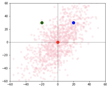
Schematic illustration of the effect of correlation on the computation of distance.

Looking at the plot  we know that the blue point is more likely to belong to the same cluster as the red point at the origin than the green point  although they are equidistant from the center. It's clear that  when there are correlated variables  we need to take the correlation into account in our distance calculation.

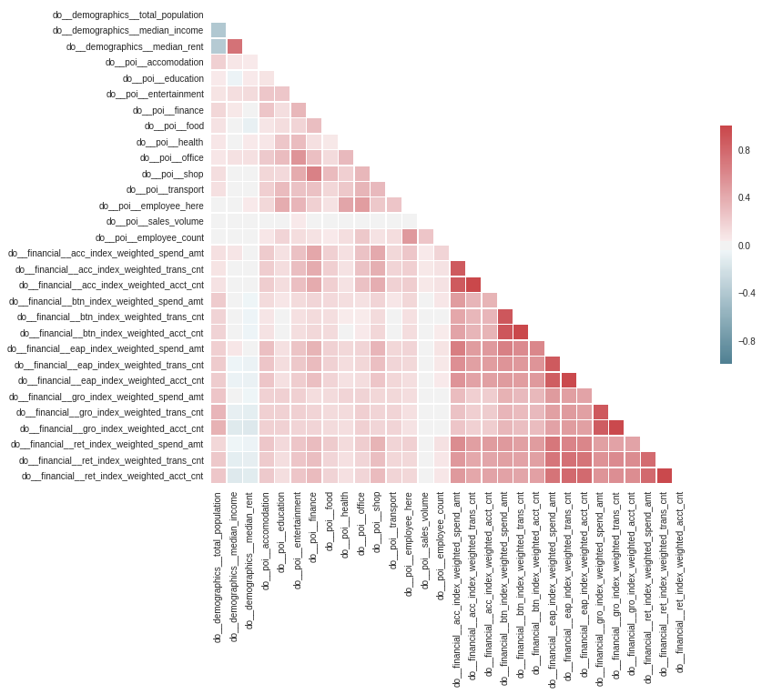
 Correlation matrix for the variables included in this analysis. Each element in the matrix represents the Pearson correlation coefficient  which is a measure of the linear correlation between two variables.

As expected  the above chart shows that a few of the variables we considered exhibit correlation (e.g. median income is positively correlated to the median rent and all financial variables are positively correlated within each other). To account for correlated variables  the distances are not computed in the original variable space but in the Principal Components Space (PCA) where the variables are linearly uncorrelated.

{::options parse_block_html="true" /}

### PCA in a nutshellPrincipal component analysis (PCA) is a technique to transform data sets of high dimensional vectors into lower dimensional ones (e.g. Ilin & Raiko  2010). This is useful  for instance  for feature extraction and noise reduction. PCA finds a smaller-dimensional linear representation of data vectors such that the original data could be reconstructed from the compressed representation with the minimum square error. The most popular approach to PCA is based on the eigen-decomposition of the sample covariance matrix

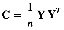
where Y is the centered (row-wise zero empirical mean) n x d data matrix  where d is the number of data points and n the number of variables. After computing the eigenvector (U) and eigenvalue (D) matrix of the covariance matrix

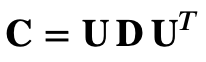
and rearranging their columns in order of decreasing eigenvalue  the  principal components (PC or factors) are computed as

where P = Up represent the eigenvectors that correspond to the largest p eigenvalues  i.e. to the largest amount of explained variance. The original (centered) data can then be reconstructed as

Here  to account for the uncertainty in the number of retained PCs  we created an ensemble of distance computations and  for each ensemble member  we randomly set the number of retained PC components within the range defined by the number of PCs explaining respectively 90% and 100% of the variance.

 Want to Become a Spatial Data Scientist? Download our free ebook!

How do we compute distances in the presence of missing data?

Unfortunately  PCA doesn't work with missing data. The vanilla solution of interpolation or imputation with means is not a great idea if missing data is common. Figure 7 shows the fraction of missing data for each variable included in this analysis. When a POI variable is missing for a given location  we can safely assume that the number of POIs for that variable in that location is zero. On the other hand  for other variables (e.g. demographics  financial) we need to find a robust method to deal with missing values.

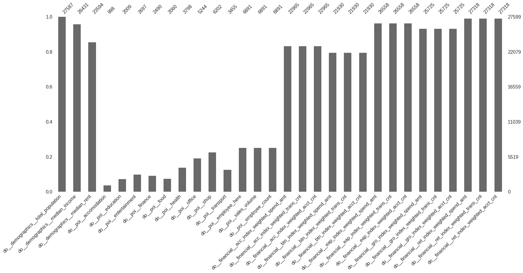
Fraction of missing data for each variable included in this analysis.

To account for missing data  here we are using a probabilistic approach to PCA  called Probabilistic PCA (PPCA  Ilin & Raiko  2010)  which uses an iterative procedure to alternatively interpolate missing data and update the uncorrelated components until convergence.

### PPCA in a nutshellIn PPCA the complete data are modelled by a generative latent variable model which iteratively updates the expected complete data log-likelihood and the maximum likelihood estimates of the parameters. PPCA also has the advantage of being faster than PCA because it does not require computation of the eigen-decomposition of the data covariance matrix. Following Ilin & Raiko (2010)  PCA can also be described as the maximum likelihood solution of a probabilistic latent variable model  which is known as PPCA:

with

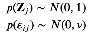
Both the principal components Z and the noise 𝜀ε are assumed normally distributed. The model can be identified by finding the maximum likelihood (ML) estimate for the model parameters using the Expectation-Maximization (EM) algorithm. EM is a general framework for learning parameters with incomplete data which iteratively updates the expected complete data log-likelihood and the maximum likelihood estimates of the parameters. In PPCA  the data are incomplete because the principal components  Zi  are not observed. When missing data are present  in the E-step  the expectation of the complete-data log-likelihood is taken with respect to the conditional distribution of the unobserved variables given the observed variables. In this case  the update EM rules are the following.

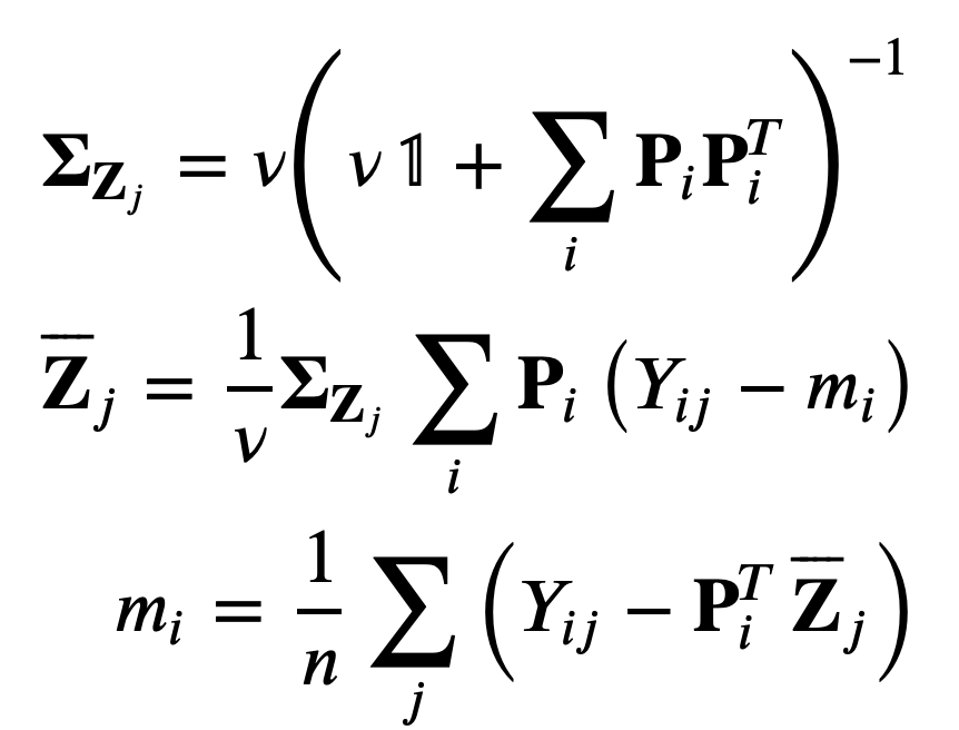
where each row of P and Z is recomputed based only on those columns of Z which contribute to the reconstruction of the observed values in the corresponding row of the data matrix.

So far we computed distances in variable space between a given shared workspace location in NY and each location in the target area in LA. We can then select the target locations with the smallest distances as the best candidates where to open/relocate offices in LA. However  how do we know that a distance is small enough  i. e.: How do we define similarity?

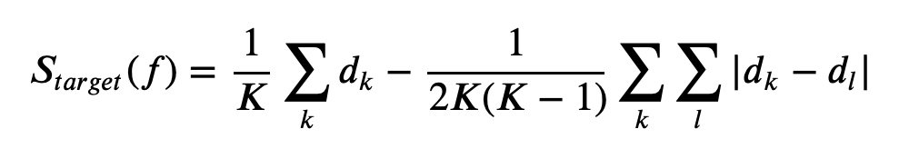
To answer this question  we defined a similarity skill score (SS) by comparing the score for each target location to the score from the mean vector data

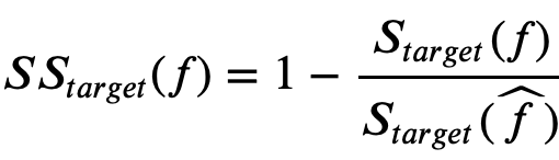
where the score just represents the distance in variable space  i.e.

If we account for the uncertainty in the computation of the distance for each target location via the ensemble generation  the score for each target location becomes

where K is the number of ensemble members.

• the Skill Score (SS) will be positive if and only if the target location is more similar to the origin than the mean vector data
• a target location with larger SS will be more similar to the origin under this scoring rule

We can then order the target location in decreasing order of SS and retain only the results which satisfy a threshold condition (SS = 1 meaning perfect matching or zero distance). More information on scoring rule can be found in Ferro (2014).

Bringing It All Together

Below we can see a map of the Similarity Skill (SS) Score for the target area for two origin location in NYC where currently there are shared workspaces  one in Manhattan and one in Brooklyn. From this plot  we can see that the method selects different target locations for the Manhattan and Brooklyn offices  which reflects the differences between the variables in the origin locations. In particular  for the Manhattan office  the selected locations in LA are clustered in the Beverly Hills and West Hollywood area  which amongst all the different areas in LA are notably the most 'similar' to Manhattan in terms of demographics  financial  and POI data. On the other hand  the locations selected as the most similar under the SS scoring rule for Brooklyn are more scattered  suggesting that our example company might consider different neighborhoods in LA when deciding to open a new office with similar characteristics to those in Brooklyn.

 Similarity Skill Score (SS) for LA locations for shared workspaces in Manhattan and Brooklyn. Only locations with SS is positive are shown.

References:

• Ferro  C. A. Fair scores for ensemble forecasts. Q.J.R. Meteorol. Soc.  140: 1917-1923. doi:10.1002/qj.2270 (2014).
• Ilin  A.  & Raiko  T.  Practical approaches to principal component analysis in the presence of missing values. Journal of Machine Learning Research  11: 1957-2000 (2010).

Special thanks to Mamata Akella  CARTO's Head of Cartography  for her support in the creation of the maps in this post.