How Socioeconomic Factors relate to Mobility during COVID-19


Since COVID-19 was first identified in Wuhan China in December 2019 the disease has spread worldwide leading to an unprecedented health and economic global crisis. In the United States (US) it spread rapidly to every state prompting non-Pharmaceutical interventions (NPIs) such as school closure and shelter-in-place (lockdown) strategies to limit intra- and inter-state mobility. While a sudden reduction in mobility following the declaration of the national emergency on March 13 and a slow increase afterwards is observed everywhere large local disparities are found between different counties.

This work from CARTO's Data Science team is intended to identify the association of such heterogeneities with the underlying socioeconomic and demographic characteristics and to provide community-level insights that could help policy evaluation and intervention.
Using a Bayesian spatial modelling framework we investigated at county level the association of these factors with changes in workplaces mobility at two points in time in the evolution of the US epidemic: the lockdown phase between the early stages of the epidemic and full shelter-at-home conditions (from February 20 2020 to April 13 2020) and the recovery phase (from April 13 2020 to July 17 2020). While controlling for the county's epidemiological situation we found that accounting for the county-level socioeconomic and demographic characteristics the model is able to explain about 40% in the variance of the changes in workplaces mobility during the lockdown phase; with larger drops in workplaces mobility observed in counties with a higher income with an older population and that are less-densely populated but with a larger density of workforce. When also accounting for the residual spatial variability the model explains about 80% of the variance; suggesting that besides socioeconomic and demographic factors neighbouring counties were similarly impacted by NPI strategies possibly driven by the state-wise regulations and their effect on neighbouring states.
Leveraging CARTO's Data Observatory
In this study we combined human mobility data with demographic data to relate the changes in workplaces mobility during the COVID-19 pandemic in the US to sociodemographic socioeconomic and business attributes at different points in time. Specifically we were interested in the heterogeneity in the response to NPI strategies in the US: for example how did changes in mobility relate to income during the lockdown phase? Did NPI strategies affect differently industrial and rural areas? Did the relationship between changes in mobility and demographic and socioeconomic factors depend on the phase of the response for example during strict lockdown or when restrictions are progressively relaxed?
We used CARTO's Data Observatory to access the Sociodemographics and Business Counts datasets from Applied Geographic Solutions (AGS). Demographic and socioeconomic attributes comprise variables such as population counts total and by age and gender household income etc. while business-related attributes refer to variables like the number of employees total and by business category etc. Extensive variables (i.e. those for which the value for a block can be viewed as a sum of sub-block values as in the case of population) were converted into densities by normalizing by the county's total population.
As a proxy for population-level movements human mobility data was obtained from Google's COVID-19 Community Mobility Reports which report daily anonymized aggregated data to track movement trends over time by geography across different categories such as workplaces retail and recreation places groceries and pharmacies parks transit stations and residential areas. The data represents the percentage change compared to a baseline defined as the median value for the corresponding day of the week during the five-week period of January 3 - February 6 2020. To capture the response of different components of the society to NPI strategies we selected as the mobility exposure of interest the changes in workplaces mobility which is expected to vary significantly across different communities.
For the Epidemiological data we used the Summary Cases dataset with county level data on the number of reported COVID-19 cases as derived from the Corona Data Scraper initiative.

Deriving the temporal limits of the lockdown and recovery phases from mobility data
The workplaces mobility data were first pre-processed to impute missing data and then smoothed to remove the high frequency variability and the weekly cycles. We included the data between February 20 (before NPI strategies were put in place) up to July 17 2020. Only counties for which the workplaces mobility had gaps of missing data shorter than three consecutive days were retained with the missing daily data imputed using linear interpolation. To isolate the low-frequency dynamic only the mobility data were then smoothed by computing for each county the running average of seven days and assigning the value to the central point.
The figure below shows for the US median and a random sample of 100 counties the time series of the percentage daily change for the imputed mobility data with and without smoothing. As expected since the national state of emergency was declared on March 13 2020 the workplaces mobility has been decreasing up to mid of April 2020 and then started to increase again for all the counties included in the random sample as well as the US median. Given the imputed and smoothed time series for each county the lockdown period was identified as the period starting from the beginning of the selected period (February 20 2020) to the April 13 2020 which corresponds to the maximum decrease in workplaces mobility for the US median. The remaining period was then identified as the recovery phase with the workplaces mobility slowly increasing again.
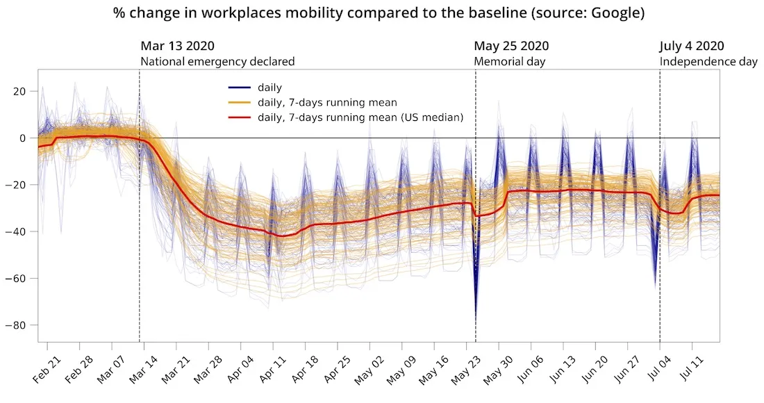
Percentage change in workplaces mobility over time with respect to the baseline February 20 2020 to July 17 2020 (source: Google). The baseline is defined as the median value for the corresponding day of the week during the five-week period of January 3 - February 6 2020
Finally the overall change in workplaces mobility for each phase and county was computed as the difference between the maximum and the minimum in the smoothed percentage change within each phase. The maps below show the overall percentage change in workplaces mobility in the lockdown and recovery phase together with the cumulative number of COVID-19 reported cases as of the last day of each phase (April 13 and July 17 2020).
Percentage change in workplaces mobility by county for the lockdown (top left) and recovery (top right) phase and the corresponding cumulative COVID-19 cases per 100 000 people as of the last day of each phase (bottom left) and (bottom right).
Building the statistical model
To model the change in mobility as a function of the Census and the epidemiological covariates we used a Generalized Linear Model (GLM) [1] within a Bayesian framework which allows to quantify the uncertainty in the estimated parameters with probability.
Due to strong pairwise correlations between the county-level census variables and to address missing data in the census covariates Principal Component Analysis in its probabilistic formulation (PPCA) [2] was first used to extract six constructs that explain 55% of the variance in demographic socioeconomic and business attributes: 'workforce density' 'density of households' 'income' 'age' 'density of Hispanic population' and 'density of non-Hispanic multiple-race population' as illustrated by the Figure below which shows the correlations between the five variables most highly correlated with each principal component score.
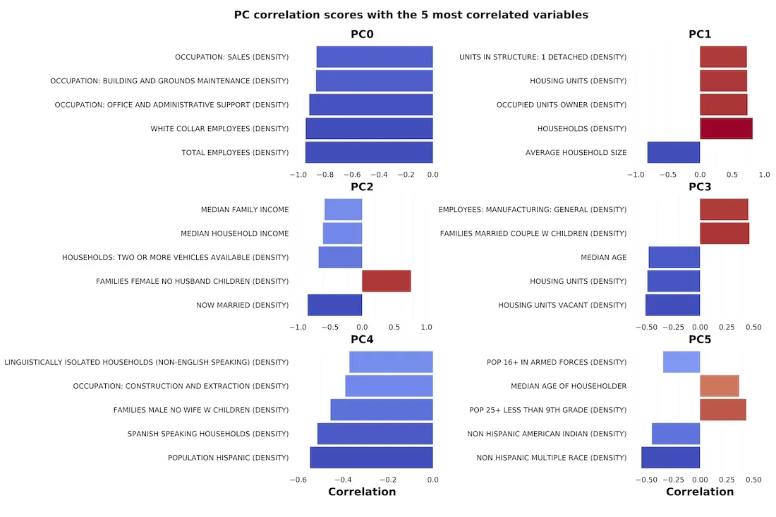
Correlations between the five variables most highly correlated with each principal component score and the corresponding principal component score from the PPCA analysis of 120 variables.
The following figure shows the retained principal component scores by county together with the sign of the correlation with the variable which better represents each construct (selected amongst the five variables most highly correlated with each principal component score).
Correlations by county between the variable which better represents each construct (selected amongst the five variables most highly correlated with each principal component score) and the corresponding principal component score from the PPCA analysis of 120 variables.
Next we fitted separately for each phase a Bayesian generalized linear regression model using a Beta likelihood and the derived constructs from the principal component analysis as fixed covariates (the Beta-model from now on). A second model also accounting for an extra spatial random effect [3] to model the dependence between counties (i.e. nearby regions are expected to have similar values for the change in workplaces mobility) was also considered (the spatial Beta-model from now on). In this context the models with and without the spatial term are complementary: while the first Beta-model can be used to estimate the coefficients of the fixed effects the second one can be used to determine if the extra-beta variability can be explained by neighbourhood effects. When the extra-beta variability can be explained by spatial dependencies the spatial model is expected to have a higher accuracy. Additionally some variations in the model coefficients are expected when the spatial random term is added to the linear predictor due to the possible confounding of the random terms and the fixed effects [4] with large variations in the model coefficients being a symptom of poor model identifiability.
Want to see this in action?
Request a live personalized demo
Analyzing the results
Model performance
The table below shows the performance of the models described in the previous section. We can see a big difference in the performance of the Beta-model in both phases. While for the lockdown phase it is able to explain about 40% of the variance in the changes in workplaces mobility this value drops to about 10% for the recovery phase. A higher accuracy in the predictions is obtained with the spatial Beta-model with pseudo-$R^2$ scores of about 0.8 for both the lockdown and the recovery phase. This clearly shows that considering neighborhood effects considerably improves the model ability to explain mobility variations per county which stresses the importance of adding a spatial component to the model for prediction tasks when dealing with spatial data.
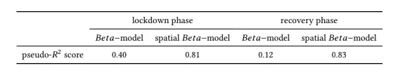
Considering neighborhood effects considerably improves the model ability to explain mobility variations per county
Effect of covariates on workplaces mobility
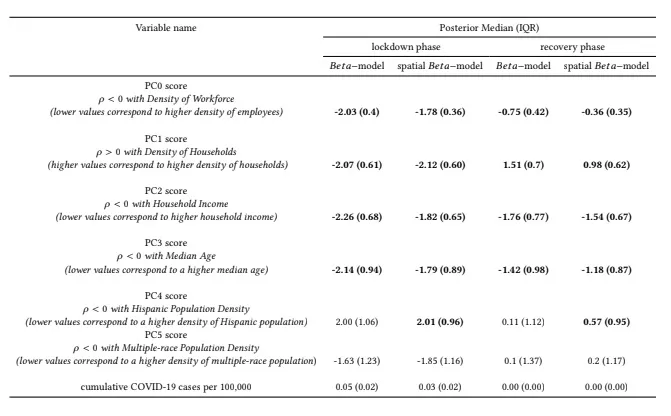
The following table reports the odds percentage relative change for 1-unit additive increase in the corresponding principal component score. As this table shows accounting for neighbourhood effects in the model does not affect significantly the contribution of the fixed covariates: the posterior median of the odds percentage relative change (as well as of the model coefficients not shown) for the Beta-model lies between the 25th and 75th percentiles estimates for the spatial Beta-model and vice versa.
These figures show that during the lockdown phase larger drops in workplaces mobility were observed in counties with a higher income with an older population and that are less-densely populated but with a higher density of workforce. Interestingly enough counties with lower Hispanic population density observed larger drops while the density of multiple-race population had a positive sign effect on workplaces mobility.
Similarly during the recovery phase larger increases in workplaces mobility are observed in counties with a higher income with an older population and a larger density of workforce. However compared to the lockdown phase the sign of the effect of the principal component score related to household density (PC1) differs observing higher increases in workplaces mobility in counties with higher density of households. An interesting insight is the little effect that the density of Hispanic and multiple-race population had on workplaces mobility during this phase.
How socioeconomic and demographic factors have influenced mobility changes during the COVID-19 US pandemic
The results of our study indicate that the different levels of decline in workplaces mobility observed during the lockdown phase were associated with the county's socioeconomic demographic and epidemiological characteristics but these factors only played a marginal role in the following period when workplaces mobility started increasing again (recovery phase). On the other hand throughout the analysis period neighbouring counties showed similar patterns in changes in workplaces mobility possibly due to state-wise regulations and their effect on neighbouring states.
During the lockdown phase larger drops in workplaces mobility were observed in counties with a higher income with an older population and that are less-densely populated but with a larger density of workforce. This result reflects the high socioeconomic and demographic disparities in the US response to the pandemic: younger lower-income and more densely populated counties responded very differently to stay-at-home orders than older and richer counties. Given that the dominant routes of transmission of SARS-CoV-2 are via respiratory large droplets communities that are less likely to be able to adapt to social distancing strategies are also more likely to get infected and contribute to the spread of the disease [5].
While the variability in the outcome explained by the constructs derived from the socioeconomic and demographic attributes is much lower similar associations are found in the recovery phase: larger increases in workplaces mobility are observed in counties with a higher income with an older population and a larger density of workforce. On the other hand higher increases in workplaces mobility are associated with counties with higher density of households and lower household size: while families with children followed more promptly lockdown restrictions they are now struggling to recover their daily mobility patterns with the easing of these restrictions while schools remained closed.
Socioeconomic demographic and epidemiological factors had a stronger influence in mobility during the lockdown phase than in the recovery phase
Although this framework only detects correlations and not causal relationships this analysis provides evidence that the observed changes in workplaces mobility affected differently US counties with different socioeconomic characteristics. By combining community-level attributes and mobility data we are able to understand at the population level the impact on mobility of income employment type epidemiological conditions as well as neighbourhood effects. While population-level analysis could be biased by unobserved confounders and should not be extrapolated to individuals nevertheless these results could help policy evaluation and intervention which especially during a state of alert are often targeted at a community level.
Want to get started?
References
[1] Nelder J. A. and Wedderburn R. W. M. Generalized linear models. Journal of the Royal Statistical Society Series A 135 3 (1972) 370–84.
[2] Ilin A. and Raiko T. Practical approaches to principal component analysis in the presence of missing values. Journal of Machine Learning Research 11 66 (2010) 1957–2000.
[3] Rue H. and Held L. Gaussian Markov Random Fields. New York: Chapman and Hall/CRC.
[4] Hodges J. S. and Reich B. J. Adding spatially-correlated errors can mess up the fixed effect you love. The American Statistician 64 4 (2010) 325–334.
[5] Hamada S Badr Hongru Du M. M. E. D. M. M. S. and Gardner L. M. Association between mobility patterns and COVID-19 transmission in the usa: a mathematical modelling study. The Lancet Infectious Diseases 0 (2020).
[6] Chen Y. and Jiao J. Relationship between socio-demographics and covid-19: A case study in three texas regions. SSRN (2020).
 | This project has received funding from the European Union's Horizon 2020 research and innovation programme under grant agreement No 960401. |