Retail Revenue Prediction Models with Spatial Data Science

As we round the corner into the latter half of 2019 the retail apocalypse continues. Business Insider is projecting more than 8 000 store closures in 2019 with major brands like Gap Walgreens Pier 1 Sears and Victoria's Secret on the list. The industry is also set to see one of the largest retail liquidation events in history with Payless announcing the closure of all 2 500 of its stores.

1. Introducing SDS to Cancel the Retail Apocalypse

In an industry under threat from thinning margins and looming ecommerce retailers hoping to not just survive but thrive need to arm themselves with more advanced business tools techniques and tactics. Being able to predict store revenues is critical allowing retail leaders to stay agile make informed decisions around current store operation and plan the most effective new openings. Leveraging Spatial Data Science allows these leaders to stay ahead of the competition and continue to grow.

In this blog post we will focus on:

• Gaining more insights from current retail store locations with Enriched Spatial Features.
• Training a Spatial Predictive Model to predict the annual revenue per store.
• Understanding the Important Features for determining revenue and how they influence the revenue predictions.
• Computing Projected Revenues at prospective store locations.

To illustrate our work we will focus on the store locations from one of the largest retailers in the US.

In order to perform our analysis we first need annual revenue data for each of the stores so that the predictive model can be trained and tested. As we did not have such a dataset at hand for all the stores in the case of this example we simulated one using data available online on the annual store revenues of that particular retailer and then modeled that metric at each location depending on other available variables such as population household income presence of competitors credit card transaction data among others. We then added spatial random effects and random noise at each location.

The following map shows the distinct store locations and the simulated annual revenue at each existing store:

2. Enrichment with location data streams

To train a Spatial Predictive Model not only do we need to know where the stores are located and how much annual revenue each store generates (i.e. our response variable) but also we should compute spatial features (i.e. independent variables) that provide us with more information on the local surroundings of each store.

For data enrichment we take advantage of the location data streams available in CARTO's Data Observatory and the enrichment toolkits available in CARTOframes so that we can easily bring in features from socio-demographic human mobility financial and other data categories.

In this exercise we use the following data streams as part of the enrichment process:

• US Census
• Consumer spending and retail potential
• Points of Interest
• Financial
• Human Mobility
• US Road Network
• Competitor locations

In order to include information about the surroundings of each store we generate the 10-minute drive isochrone for each store location.

The above map shows 10-minute drive isochron buffers for retail stores near Kansas City MO and Kansas City KS.

Then we run a spatial join between each isochrone and the spatial features from the different location data streams. With our data newly enriched by these features we are able to get a better sense of what the surroundings look like for different stores. As an example the following map shows the consumer spending in department stores by the households located in the surrounding of each of our retailer's stores (aggregated at store level).

After this Data Enrichment phase we are able to give an answer to questions such as: "how many people live within the 10-minute driving isochrone of each store and what is their average household income?" "how many competitors are located within the surroundings of the store?" "how many restaurants leisure centers parks are within that buffer? "what's the average ticket size in the area?" "how many interstate roads intersect with the isochrone? etc.

3. Building a Predictive Model

Now that we have enriched the information that we have about each of the stores and their locations with more features we will start the workflow of building a model that allows us to predict the revenue at each store and also to predict the potential revenue of a store in a location in which the retailer does not have a presence. The logic that we will follow on this workflow is to start with data pre-processing feature selection to simplify and train ensemble models tuning hyperparameters and finally implementing regression kriging to improve the prediction capabilities of the model.

Data Pre-processing

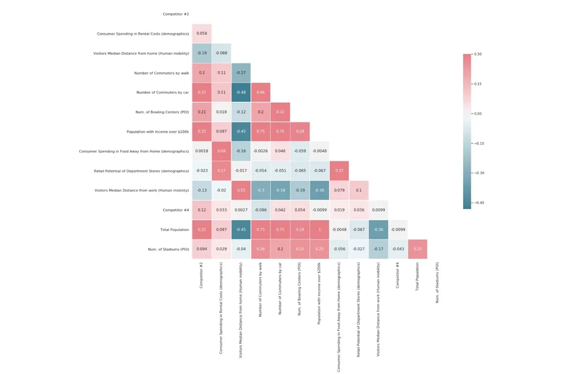
Before we start to build a spatial model it's essential to conduct a data preprocessing phase in order to: fill-in missing data convert different data types and standardize and normalize the features if necessary. In addition as Occam's Razor states "More things should not be used than are necessary " we also run a feature selection step to make sure we are not considering redundant features and to avoid the "Curse of Dimensionality" (i.e. as the number of features or dimensions grows the amount of data we need to generalize accurately grows exponentially). Feature selection also helps us enhance the interpretability of the results and shorten the runtime. We can see the correlation matrix of subsets of features below.

There are several feature selection methods that we can use for this phase of the workflow:

• LASSO (Least Absolute Shrinkage and Selection Operator) [1]
• Stability Selection [2]
• Boruta [3 4]

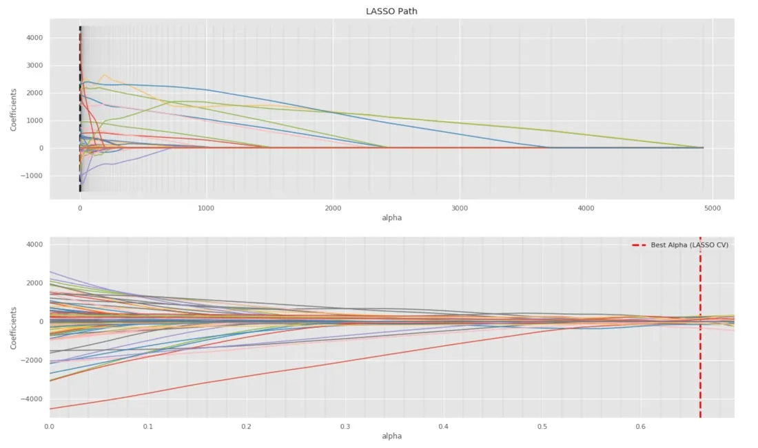
LASSO is a regression analysis method that performs both variable selection and regularization in order to enhance the prediction accuracy and interpretability of the statistical model. In the plot below we can see the performance of LASSO for the features available for our model. In this plot each line represents one feature. With regularization intensity going up from right to left more features are filtered out (i.e. feature lines reach the coefficient zero point). In the second plot we have used cross-validation to find the best regularization hyper-parameter (i.e. alpha). Finally we select the features which have a non-zero coefficient for the best alpha.

The idea of Stability Selection is to inject more noise into the original problem by bootstrapping samples of the data and then to use LASSO to find out which features are important in every sampled version of the data. The results on each run are then aggregated to compute a stability score for each feature in the data and then features are selected by choosing an appropriate threshold for the stability scores.

As an alternative Boruta is an "all-relevant" feature selection method while the other methods are "minimal optimal". This means that Boruta tries to find all features carrying information usable for prediction rather than finding a compact subset of features on which some classifier method has minimal error.

Spatial Modeling

To start modeling we first need to split the full dataset into two parts: Training data (70%) and Test (30%) data. Test data will be used to evaluate the results of the model when using the training data.

At the first step of the modeling section we fit the data into two ensemble models with the selected features from the previous step:

• RandomForest
• Gradient Boosting Regression

We compare the model performances by calculating the following metrics with the Test data:

$$R^{2}$$ (R-squared or Coefficient of determination) = $$1-{\sum {i}(y{i}-y_pred_i)^{2} \over \sum {i}(y{i}-{\bar {y}})^{2}}$$

$$R^{2}$$ is the proportion of the variance in the dependent variable (i.e. annual revenue) that is predictable from the independent variable(s). It provides a measure of how well observed outcomes are replicated by the model based on the proportion of total variation of outcomes explained by the model. In this case the higher the better the model is.

$$RMSE$$ (Root Mean Square Error) = $$\sqrt{\frac{1}{n}\Sigma_{i=1}^{n}{\Big(y_pred_i -y_i\Big)^2}}$$

RMSE (Root Mean Square Error) is a frequently used measure of the differences between the values predicted by a model and the values observed. In this case the lower the better the model performs.

In this case we observe a higher performance with the RandomForest model as it shows R2 = 0.672 and RMSE = 3788.467 versus R2 = 0.593 and RMSE = 4222.086 obtained with the Gradient Boosting Regression.

Continuing with the RandomForest we then apply Bayesian HyperParameter Optimization [5] to enhance its predictability. We concentrate on three common hyperparameters for ensemble models: min_samples_leaf max depth and the number of estimators.

With the new optimal hyperparameter values we fit the data into the model again. As a result our RandomForest model performs at R2 = 0.726 and RMSE = 3461.90 which shows improvement compared with the model at the previous step.

We also want to explore whether there's any spatial randomness in the model's residual so that we can add prediction of spatial random effect in the regression model to increase its performance. In order to do that we generate the semivariogram to detect whether the residuals in the model are related with spatial locations. From the result we can learn that store locations with smaller pairwise distances (smaller lag) tend to be more similar in terms of spatial randomness (i.e. smaller semivariance) which means that in the annual revenue data per store exists a spatial pattern.

To predict the spatial randomness affecting the annual revenues we implement a method called Regression Kriging [6]. It is a spatial interpolation technique that combines a regression of the dependent variable with simple kriging of the regression residuals. The advantage of Regression Kriging is the ability to extend the method to a broader range of regression techniques and to allow separate interpretation of the two interpolated components.

We sum up the Spatial Kriging Value to the prediction value obtained by the RandomForest with Hyperparameter Tuning. With the RandomForest model after hyperparameter tuning and regression kriging we obtain R2=0.766 and RMSE=3199.036 which means the model performance as improved even further compared to the previous steps.

Model Interpretation

Now that we have built the predictive model we want to understand which of the features are more important in order to do that we generate a feature importance table.

In detail for each Decision Tree Regressor in the last model we calculate the Node Importance (NI) as for node j
$$NI_j=w_jC_j − w_{left(j)} C_{left(j)}−w_{right(j)}C_{right(j)}$$

where

• $$w_j$$ is weighted number of samples in node j
• $$Cj$$ is impurity in this node (Here Mean Square Error)
• $$left(j)$$ and $$right(j)$$ are its respective children nodes.

Then feature importance (FI) of feature i in a specific Decision Tree Model is computed as:

$$FI_i = \frac{\sum_{j : \text{node j splits on feature i}} NI_j}{\sum_{j \in \text{all nodes}} NI_j}$$

The final feature importance of feature i is computed as the average feature importance of all Decision Tree Estimators in the RandomForest Model.

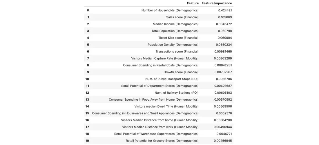
From the list we can see which of the features from different location data streams are more relevant to our revenue predictions. We observe that features from demographic and financial data rank higher in terms of importance in our model. Features from POIs and Human Mobility such as the number of public transportation stops the visitor capture rate and the visitor dwell time also play important roles.

Another tool for model Interpretation is SHapley Additive exPlanations (SHAP) [7 8 9]. SHAP is a unified approach to explain the output of any machine learning model and its values show the consistent locally accurate and individualized attribution of each feature in the model. In this exercise SHAP helps us understand in which way each feature affects the prediction record by record (see the SHAP Summary plot below).

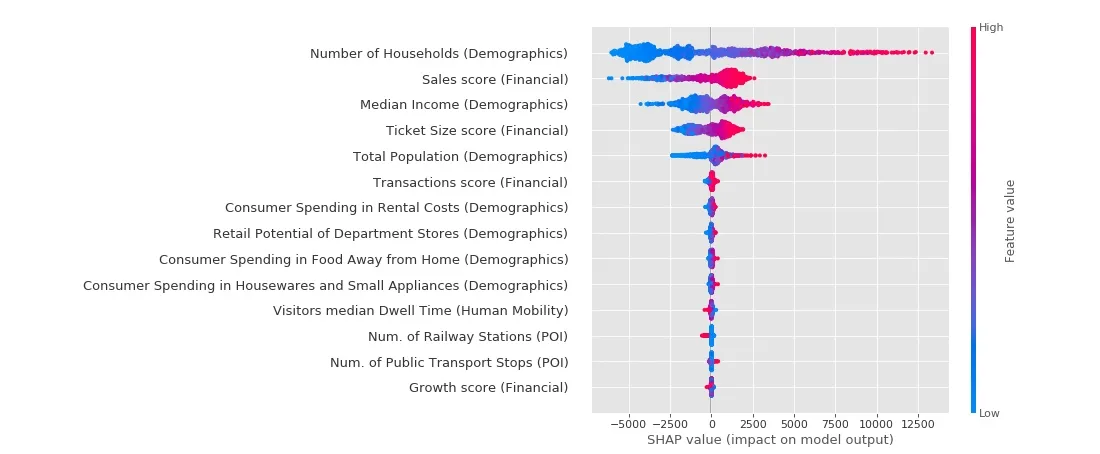
The plot mainly demonstrates that with feature values increasing or decreasing the magnitude and direction of feature impact on the model output may change accordingly. For example having a high Number of Households is associated with high and positive impact on model output. Besides credit card sales scores tend to have a positive influence on stores located in areas with high feature values but would cause a negative impact on stores with lower values.

With SHAP we can also see at single record level how each feature makes a contribution (negative/positive) to the prediction value.

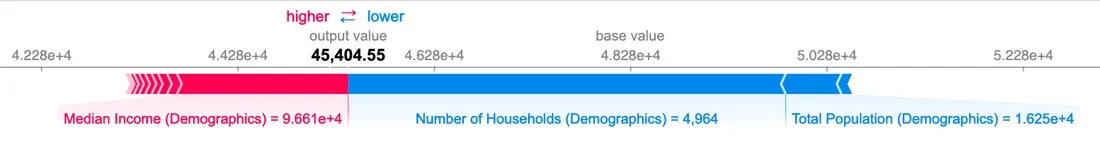
The above example shows for one specific store how features contribute to push the model output from the base value (i.e. the average revenue over the training dataset) to final predicted value. Features pushing the prediction higher are shown in red those pushing the prediction lower are in blue. Focusing on this store we can see Median Income = 96610 (in contrast to Average Median Income = 62411) pushes the predicted revenue going higher from the base value and Number of Households = 4964 which is much lower than mean value = 18001 makes the model output go down.

4. Applying Revenue Predictions

Finally it is time for us to start using our model for predicting revenues at potential new retail locations. In order to do that we define a list of 40 potential sites in which the retailer may want to consider opening a new store and we enrich their 10-min drive isochrones with features from the location data streams as we have done in Section 2 when building our model. We then apply the resulting model in Section 3 to generate predictions for annual revenues at the different candidate locations. Note that to do that we only need to repeat data enrichment workflow as we did before. The Map below shows the projected revenues for potential store locations in Los Angeles California.

From the revenue predictions we observe that the top performant new potential stores are located in Los Angeles happen to be in areas where financial sales score and ticket size score as well as number of household and median household income are much higher. Besides potential locations with higher predictions tend to have higher capture rate from human mobility's perspective.

5. Conclusion

Modern retail is a challenging field with ecommerce narrowing margins across nearly every category. Retailers need to be using every tool at their disposal to inform their site-planning and operational decisions and protect their bottom line.

By leveraging the latest tools and techniques such as enriching existing sales data with modern data streams and creating predictive models that incorporate spatial components equips business leaders with the insights they need to act intelligently decisively and quickly.

6. References

1. Tibshirani Robert. "Regression shrinkage and selection via the lasso." Journal of the Royal Statistical Society: Series B (Methodological) 58.1 (1996): 267-288.
2. Meinshausen Nicolai and Peter Bühlmann. "Stability selection." Journal of the Royal Statistical Society: Series B (Statistical Methodology) 72.4 (2010): 417-473.
3. Kursa Miron B. and Witold R. Rudnicki. "Feature selection with the Boruta package." J Stat Softw 36.11 (2010): 1-13.
4. BorutaPy – an all relevant feature selection method http://danielhomola.com/2015/05/08/borutapy-an-all-relevant-feature-selection-method/
5. Snoek Jasper Hugo Larochelle and Ryan P. Adams. "Practical bayesian optimization of machine learning algorithms." Advances in neural information processing systems. 2012.
6. Hengl Tomislav & Heuvelink Gerard & Rossiter David. (2007). About regression-kriging: From equations to case studies. Computers & Geosciences. 33. 1301-1315.10.1016/j.cageo.2007.05.001.
7. Lundberg Scott M. Gabriel G. Erion and Su-In Lee. "Consistent individualized feature attribution for tree ensembles." arXiv preprint arXiv:1802.03888 (2018).
8. SHAP (SHapley Additive exPlanations) https://github.com/slundberg/shap
9. Lundberg Scott M. et al. "Explainable machine-learning predictions for the prevention of hypoxaemia during surgery." Nature biomedical engineering 2.10 (2018): 749.

Special thanks to Mamata Akella CARTO's Head of Cartography for her support in the creation of the maps in this post.