Using Spatial Composites for Climate Change Impact Assessment

Assets such as infrastructure, buildings, and natural resources are critical to human society and economic growth. Climate change can have severe consequences on these assets, including damage from extreme weather events, sea-level rise, and shifting precipitation patterns. If these impacts are not adequately assessed and managed, they can lead to significant financial losses, social disruption, and environmental degradation. 

Climate change is a complex and dynamic process influenced by various natural and human factors, such as greenhouse gas emissions and urbanization. It is also a global phenomenon, with effects that might affect distinct regions differently, making it difficult to develop accurate and localized risk models. To effectively create precise climate change risk models, companies and stakeholders need to be able to access relevant data sources and tools. 

In this blog post, we have partnered with The Climate Data Factory to showcase how to assess the risk associated with climate change for different types of assets, such as buildings, Points of Interest (POIs), roads, etc. To do this, we will take advantage of a new feature of CARTO Analytics Toolbox for BigQuery to compute spatial composite scores. These represent aggregated information that can be used to define complex and multidimensional concepts that cannot be measured directly, such as  the risks associated with climate change. 

Composite scores can be a valuable approach in climate change risk modeling,overcoming data limitations, simplifying modeling efforts, capturing spatial heterogeneity, facilitating decision-making, and providing scalability and flexibility.

To assess the risks different assets may be exposed to as a result of a changing climate, we considered the following data:

• Climate indices: 2081-2100 averages for different climate indices measuring extreme temperature and precipitation conditions - as well as for long-term changes in essential climate variables such as temperature and humidity from The Climate Data Factory (TDCF). TCDF offers multi-model and multi-scenario, ready-to-use climate data, which are suitable for direct use in climate change impact studies and physical risk assessments. These are available on demand and directly from our Data Observatory for a selection of variables and spatio-temporal resolutions. 
• Sociodemographic, urbanity and POI-related information from CARTO Spatial Features‍
• USA Road network data curated by CARTO, which offers access to OpenStreetMap's highways organized by speed profile for different modes of transportation. These features have been divided into segments that have been built to form the edges of a connected graph.

Climate change can increase disaster risk by modifying the frequency and intensity of hazards, affecting vulnerability and exposure patterns. To model different types of climate hazards, we’ll start by deriving two different risk scores:

• Chronic Hazard Risk Score:  reflects the risk associated with long-term shifts in mean climate conditions (e.g. increased global summer temperatures). Here we will compute this score by taking into account the long-term changes to the mean temperature and relative humidity, with extreme heat paired with high humidity posing a substantial threat to life Anomalies over the 2081-2100 period for these variables were computed with respect to 2001-2020 averages.
• Acute Hazard Risk Score:  quantifies the changes in the frequency and intensity of extreme events as a result of changes in their distribution (e.g. longer and more frequent intense rainfall), including shifts in the mean. For this blogpost, we will consider the risk associated with extreme precipitation (long wet periods and high precipitation), based on 2081-2100 averages for the number of consecutive wet days periods, and the percentage of very wet days.

To analyze climate-related risks at the asset level, these hazard scores can be then combined with other indicators that take into account the level of exposure and the vulnerability of specific assets.

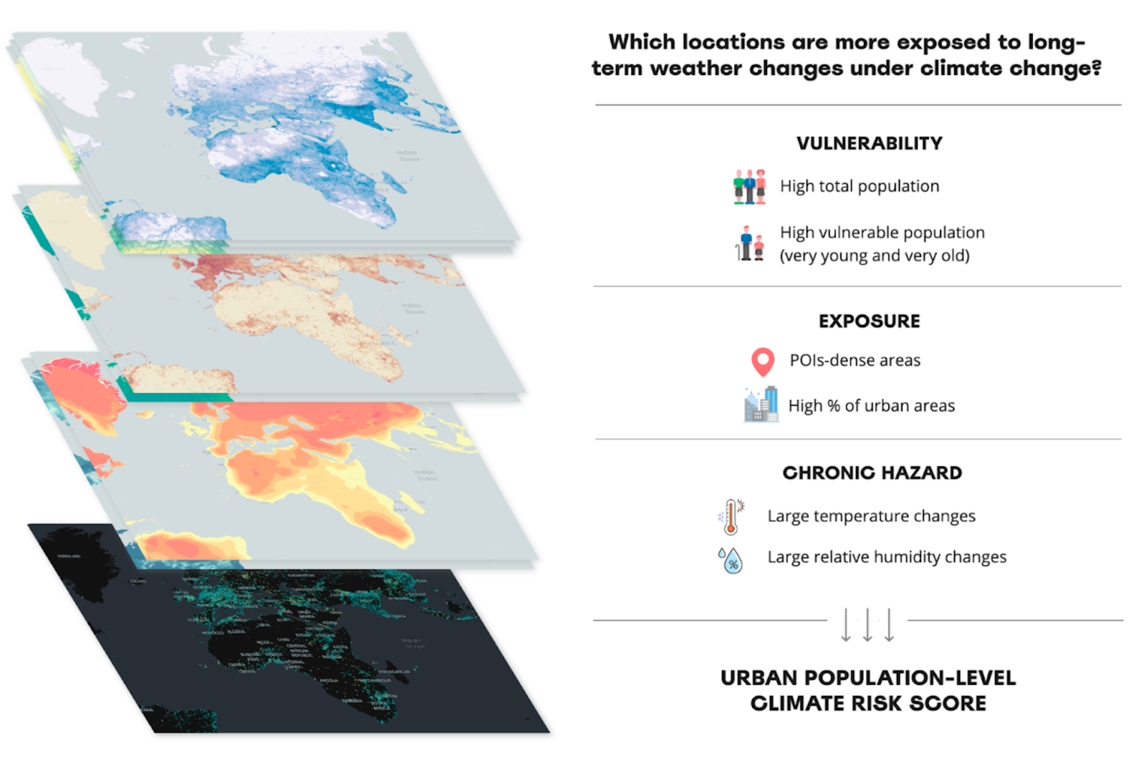
We will start by deriving a composite score to assess the chronic risk at the population level, focusing only on urban areas, which are home to the majority of the Earth’s population. By leveraging this information, governments can take proactive measures to address climate change and build more resilient communities by increasing awareness, guiding urban expansion and efficiently allocating resources to face climate impacts. 

This score will be computed by multiplying the Chronic Hazard Risk Score  by the sum of an Exposure Score, accounting for the level of built-up areas and the presence of POIs (as a proxy for urban infrastructure) and a Vulnerability Score, which represents the likelihood of damage due to exposure to a climate hazard, both in terms of sensitivity to the negative impacts of climate change and the ability to adapt. While for the hazard score we will compute one global composite score, both the exposure and vulnerability will be calculated country by country to account for the inter-country variations in sociodemographic and infrastructure patterns.

Apart from the physical risks, assets will be exposed to financial risks associated with the transition to a low-carbon economy, as governments and businesses seek to mitigate climate change. For example, a transition to net-zero emissions would entail much greater demand for electric vehicles and the underground cabling could be exposed to the effects of extreme heat and flooding. Similarly, to reduce emissions, mobility and transportation companies might be required to put in place new strategies to optimize fleets, which could also be affected by extreme weather events through reduced visibility, speed, increased stopping times, etc. As a second example, we will therefore assign the Acute Hazard Risk Score to the US road network, and show how the derived score can help develop mitigation strategies to adapt the current road network to extreme precipitation events driven by climate change.

All composite scores are derived using the Analytics Toolbox for BigQuery procedure CREATE_SPATIAL_COMPOSITE_UNSUPERVISED, which provides a set of methods to combine multiple input variables, scaled and weighted accordingly, into a meaningful score. Depending on the variables used as inputs and the type of score, different methods can be used. You can refer to the Technical note at the end of this blogpost for more details on how each composite score was  computed, and why specific parameters have been selected.

The map on the top panel shows the overall risk associated with long-term changes with respect to current conditions in temperature and humidity to people living in urban areas. In hot and humid conditions, the human body can no longer cool itself by evaporating sweat from the surface of the body, with prolonged exposure to such conditions posing a threat especially in very dense built up areas. There, the cooling effect from the vegetation is reduced and vulnerable populations such as the young/elderly and those with chronic diseases are more prone to suffer serious consequences of climate change.

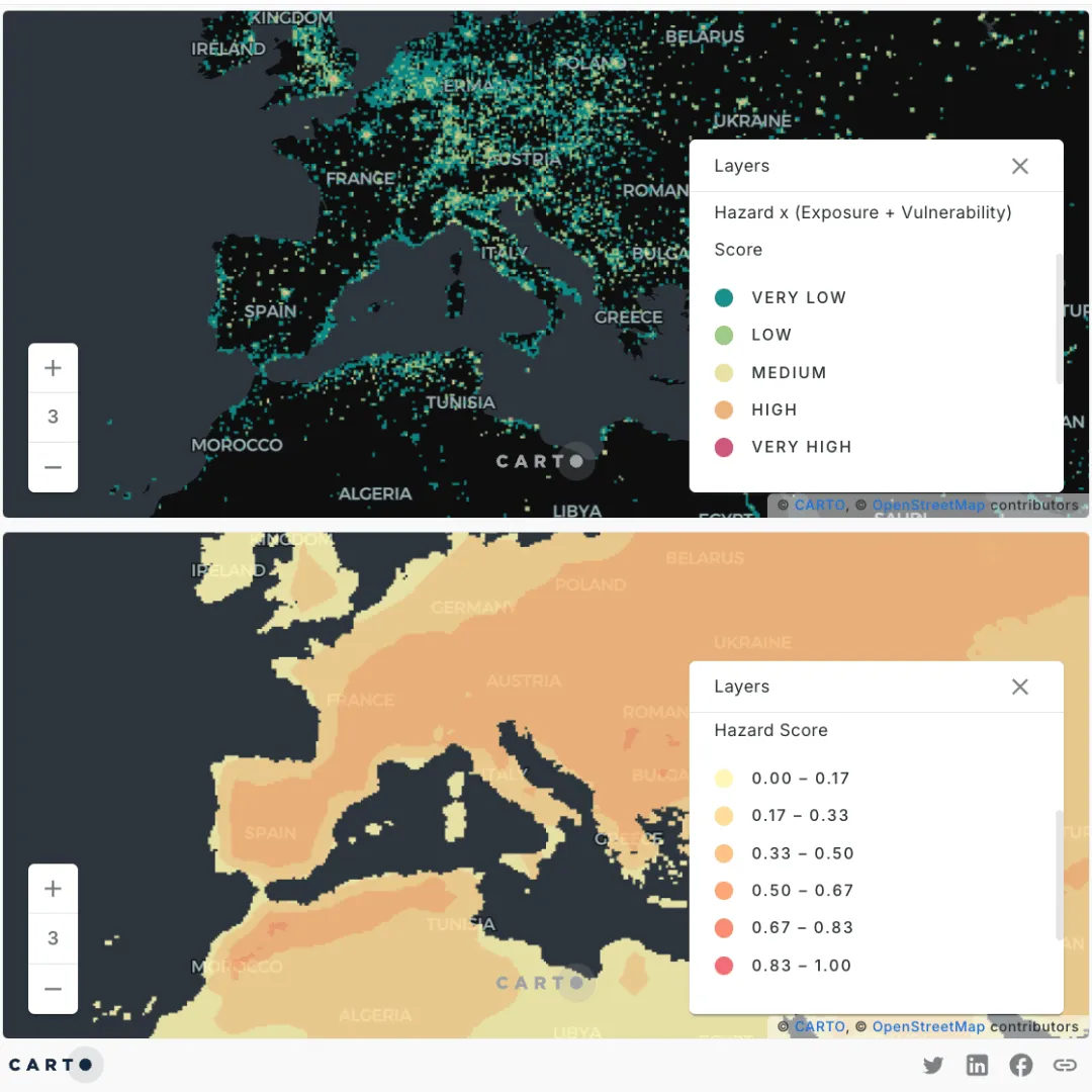
As shown in the map, for each country, a greater climate risk is associated with highly-populated urban regions, such as big city centers, and areas with more extreme changes compared to the current conditions (a.k.a larger anomalies), where the effects of long-term shifts in weather conditions will have a greater impact on society. On the other hand, as shown by the bottom panel, remote and rural areas with a high hazard risk (e.g. northern territories in Canada or the central Amazon), are not reflected in the overall risk since the hazard won’t directly affect the population living in those areas.

However, when informing global policy and decision making, impacts on the environment might still be relevant to urban communities because of feedback loops (e.g.  warming in the Arctic has led to melting sea ice, which has prompted even more warming at lower latitudes). You can toggle layers on the bottom map to visualize how each sub-score contributes to the overall risk score. 

Finally, this next map shows the risk associated with extreme precipitation and flooding computed at the road-level for all major roads in the US.

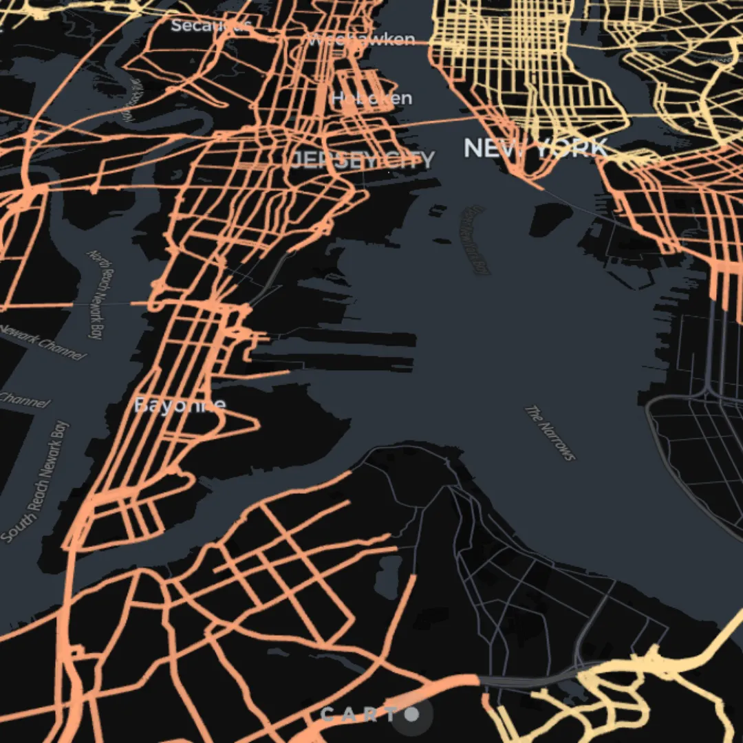
If we navigate through the map, we can see that specific roads will be more at risk than others, which helps to spot areas where both physical risks, for example associated with the quality of the asphalt, the available alternative routes, etc., and financial risks, associated with mitigation strategies, might be higher. It is particularly interesting how the risk is higher in the southern part of the US, which is known to be greatly affected by severe storms and hurricanes, especially in Florida, Louisiana and Texas, and might require more effort to prepare the road infrastructure and to increase awareness in the population.

This blogpost has shown a simplified approach to creating a composite score to measure the risk associated with climate-related hazards for different types of assets. Of course, for specific use cases, different types of data might be required. To create your own analysis and select the right data sources, you can take a look at our Data Catalog and can grab a free 14-day CARTO trial to give it a go yourself!

To compute each composite score, the following queries were executed using CARTO’s Analytics Toolbox for BigQuery procedure CREATE_SPATIAL_COMPOSITE_UNSUPERVISED. Notice that this analysis is not reproducible since in this case premium data was used.

The Acute Hazard Risk Score was derived for the US from a set of climate indexes related to extreme precipitation events provided by our partner The Climate Data Factory, as 2081-2100 averages: the number of 5-consecutive wet (consecutive_wet_days_index) days periods, and the percentage of very wet days (precipitation > 95th percentile as computed for the 1981-2010 reference period) during wet days (very_wet_days). 

 The method requires setting several parameters, including:

• scoring_method: the FIRST_PC method computes the score as the first principal component of a Principal Component Analysis and it was selected to maximize the variation in the input data.
• correlation_var: the score will be positively correlated with the variable  consecutive_wet_days_index.
• bucketize_method: the QUANTILES method is used to categorize the score into nbuckets (5) quantile-based breaks.

   
CALL `carto-un`.carto.CREATE_SPATIAL_COMPOSITE_UNSUPERVISED(
'SELECT quadbin, consecutive_wet_days_index, very_wet_days
 FROM `my-project.my-dataset.features_glo_quadbin15`
 WHERE country_iso_a3 = ‘USA’',
'quadbin', 
'my-project.my-dataset.H_acute_score_USA',
'''{
    "scoring_method":"FIRST_PC",
    "correlation_var":"consecutive_wet_days_index",
    "bucketize_method":"QUANTILES",
    "nbuckets":5
}'''
)
   

To compute the global Chronic Hazard Risk Score the FIRST_PC method is also applied, but now selecting as input variables the anomalies (a.k.a. differences) between the averages over 2081-2100 for a selection of essential climate variables and their average over the 2001-2020 reference period, with the temperature anomaly (tmp_anomaly) selected as the variable to be positively correlated with the score. Additionally, we will set the return_range parameter so that the score will be returned on a 0-to-1 scale, where 0 means less hazard and 1 states for more hazard. This same range will be used to compute all remaining composite scores.

   
CALL `carto-un`.carto.CREATE_SPATIAL_COMPOSITE_UNSUPERVISED(
'SELECT quadbin, tmp_anomaly, rh_anomaly
 FROM `my-project.my-dataset.features_glo_quadbin15`',
'quadbin', 
'my-project.my-dataset.H_chronic_score',
'''{
    "scoring_method":"FIRST_PC",
    "correlation_var":"tmp_anomaly",
    "return_range":[0.0, 1.0]
}'''
)

   

The  Exposure Score  is obtained country by country by selecting input variables that represent infrastructure presence in urban areas (we are therefore eliminating remote (0) and rural (1) areas from the analysis), such as the number of POIs within a buffer of 2.5 km (pois_lag) and urban areas (urbanity_ordinal), as well as the following parameters:

• scoring_method: with the CUSTOM_WEIGHTS method, the score is computed by first scaling each input variable and then aggregating them according to user-defined scaling and aggregation functions and individual weights. In this case equal weights will be assigned to each.
• scaling: the scaling function was set to RANKING to compute the percent rank since one of the input variables is ordinal (urbanity_ordinal). Notice that categorical variables need to be first converted to ordinal.
• aggregation: the LINEAR aggregation function will aggregate the variables linearly, which means that high values in one variable compensate for low values in others.

   
CALL `carto-un`.carto.CREATE_SPATIAL_COMPOSITE_UNSUPERVISED(
'SELECT quadbin, pois_lag, urbanity_ordinal
 FROM `my-project.my-dataset.features_glo_quadbin15`
 WHERE country_iso_a3 = 'my-country' AND urbanity_ordinal >= 2',
'quadbin', 
'my-project.my-dataset.E_score',
'''{
    "scoring_method":"CUSTOM_WEIGHTS",
    "aggregation": "LINEAR",
    "scaling": "RANKING",
    "return_range":[0.0, 1.0]
}'''
)

   

The  Vulnerability Score was derived using a similar approach as for the Exposure Score, taking into account the total (pop) and vulnerable population (pop_under_15 and pop_65_and_over) in urban areas, and by setting the following parameters:

• weights: by giving a weight of 0.2 to the total population, the remaining 0.8 is split into the other variables, which will imply a greater influence over the final score.
• aggregation: with the GEOMETRIC aggregation, high values in one variable won’t  be fully compensated with low values in others and balance between the input variables is rewarded, which is preferable when representing vulnerability. Notice that the input variable values must be strictly positive, so we will remove those cells where data is below a close-to-0 threshold.

   
CALL `carto-un`.carto.CREATE_SPATIAL_COMPOSITE_UNSUPERVISED(
'SELECT quadbin, pop_under_15, pop_65_and_over, pop
 FROM `my-project.my-dataset.features_glo_quadbin15`
 WHERE country_iso_a3 = 'my-country' AND 
 pop_under_15 > 0.001 AND pop_65_and_over > 0.001 AND pop > 0.001 AND urbanity_ordinal >= 2',
'quadbin', 
'my-project.my-dataset.V_score',
'''{
    "scoring_method":"CUSTOM_WEIGHTS",
    "aggregation": "GEOMETRIC",
    "scaling": "MIN_MAX_SCALER",
    "weights": {{"pop":0.2}},
    "return_range":[0.0, 1.0]
}'''
)

   

The risk to which an asset may be subjected to can be defined as the product of a hazard confronted to the vulnerable assets that can be exposed to that specific potential danger. 

So, to derive the Urban Population-level Climate Risk Score, we multiplied the normalized Chronic Hazard Score by the normalized sum of the Exposure and Vulnerability Scores, that represent the asset as sensitive high-populated and high-infrastructure presence areas. Then, we bucketize country by country the resulting composite into 5 equal intervals that describe the risk level of the urban asset, from ‘Very Low’ to ‘Very High’.

   
SELECT hc.quadbin, h.spatial_score * ML.MIN_MAX_SCALER(e.spatial_score + v.spatial_score) OVER() as risk_chronic
FROM `my-project.my-dataset.H_chronic_score` as h
ON feats.quadbin = hc.quadbin        
LEFT JOIN `my-project.my-dataset.E_score` as e
ON feats.quadbin = e.quadbin
LEFT JOIN `my-project.my-dataset.V_score` as v
ON feats.quadbin = v.quadbin

   

Lastly, to derive the Road-level Climate Risk Score, we assigned the Acute Hazard Score to the road network asset in the US by simply enriching the road segments with the hazard risk level information previously derived. Only major car and motorway roads were considered.

To learn more about how to integrate composite scores into your geospatial analysis, visit the CARTO Academy for resources covering data preparation, visualization, and advanced spatial analysis. Or get in touch with our expert team for a live demo!

Hear from our experts!

Request a demo