CARTO’s Ultimate Guide to Spatial Joins & Predicates with SQL


If you’re a Spatial Data Scientist there’s probably one operation type you’ll be performing all the time; maybe more than anything else. The Spatial Join. Spatial Joins are the absolute cornerstone of gaining insight from location data and are a pretty simple concept; they take data from one geography or spatial zone and attach it to another.
They’re a simple enough concept; to execute you basically need three things:
- A target dataset: this is the output geography your data will be attached to. Maybe it’s your site boundary or a Spatial Index.
- A join dataset and variables: this is the source of the data that you’ll be joining to the input dataset. It could be employment population revenue total addressable market… pretty much anything.
- A Spatial Predicate: the relationship that defines the spatial join. This will return a boolean result; if the predicate condition is true then a join occurs and if false then it does not.
In this post we’ll cover how to perform Spatial Joins and filters in SQL before running through the different spatial predicate types. This guide is aimed at newcomers to Spatial SQL or geospatial analysis in general but by the end of this post you’ll be an expert in one of the most important Location Intelligence operations - Spatial Joins!
Spatial Joins in SQL
.webp)
First of all let’s run through how to use Spatial SQL to perform a Spatial Join. If you aren’t already a CARTO user why not sign up for our two-week free trial so you can follow these examples?
The basic syntax of a Spatial Join is super simple:
SELECT *  joincalculation(aggregatefield) as newfieldname FROM targetdata
LEFT JOIN joindata
ON spatialpredicate(targetdata.geometry  joindata.geometry)
Let’s illustrate that with a simple example. Imagine we want to find out the number of airports in each US state. I’ve subscribed to Natural Earth Airports (the join dataset) and US States (the target dataset) both freely available via our Spatial Data Catalog. The variable we’re joining is simply a count of the geometry of the airports.
This is an example of a many-to-one join where we are aggregating the data from many airports to individual states. In SQL if we perform an aggregation (here being count) on one field then all other fields also need to have an aggregation performed on them.
You can use the GROUP BY function to do this for most fields. However this is unadvisable (and often won’t work) for geometry variables; for this we need to use ST_UNION_AGG() which performs a geometry union (i.e. merges all grouped features together). You’ll also see the predicate ST_CONTAINS in the code below which tests whether an airport geometry is contained by a state… keep reading to learn more about this!
Check this out below!
WITH
/*Give the datasets an alias for ease of use*/
states AS
(SELECT * FROM `carto-data.ac_lqe3zwgu.sub_usa_tiger_geography_usa_state_2019`)
airports AS (SELECT * FROM `carto-data.ac_7xhfwyml.sub_natural_earth_geography_glo_airports_410`)
/Perform the join/
SELECT
    st_union_agg(states.geom) AS geom
    states.do_label
    count(airports.geom) AS airports_count
FROM states
LEFT JOIN airports
    ON ST_CONTAINS(states.geom  airports.geom)
    GROUP BY states.do_label
Nailed it!
So that’s a simple spatial join. You can build complexity in as you need maybe incorporating transformations (such as ST_BUFFER()) or constructors such as ST_MAKEENVELOPE()).
Note: when copying code from this or any CARTO blog please note that every account’s connection will have a different series of characters following “carto-data.ac_…” You’ll need to replace these characters with your own specific connection; find this text by subscribing to a dataset and clicking “access in” or “create a map” in the Data Explorer. Find out more here!
Spatial Filters in SQL
Before we move on let’s quickly touch on spatial filters; another really common use of predicates. This is a way of filtering your data based on its relationship with another layer. The basic syntax of this is as follows:
SELECT targetdata.* FROM targetdata  filterdata
WHERE spatialpredicate(targetdata.geometry  filterdata.geometry)
So drawing on the example above let’s filter our states layer to only show those which have an airport.
WITH
/Give the datasets an alias for ease of use/
states AS
(SELECT * FROM carto-data.ac_lqe3zwgu.sub_usa_tiger_geography_usa_state_2019)
airports AS (SELECT * FROM carto-data.ac_7xhfwyml.sub_natural_earth_geography_glo_airports_410)
/Perform the filter/
SELECT states.geom  states.do_label
FROM states  airports
    WHERE ST_CONTAINS(states.geom  airports.geom)
Easy right? In both of these examples we’ve used the predicate ST_CONTAINS but there is a whole world of other spatial predicates out there which brings us to…
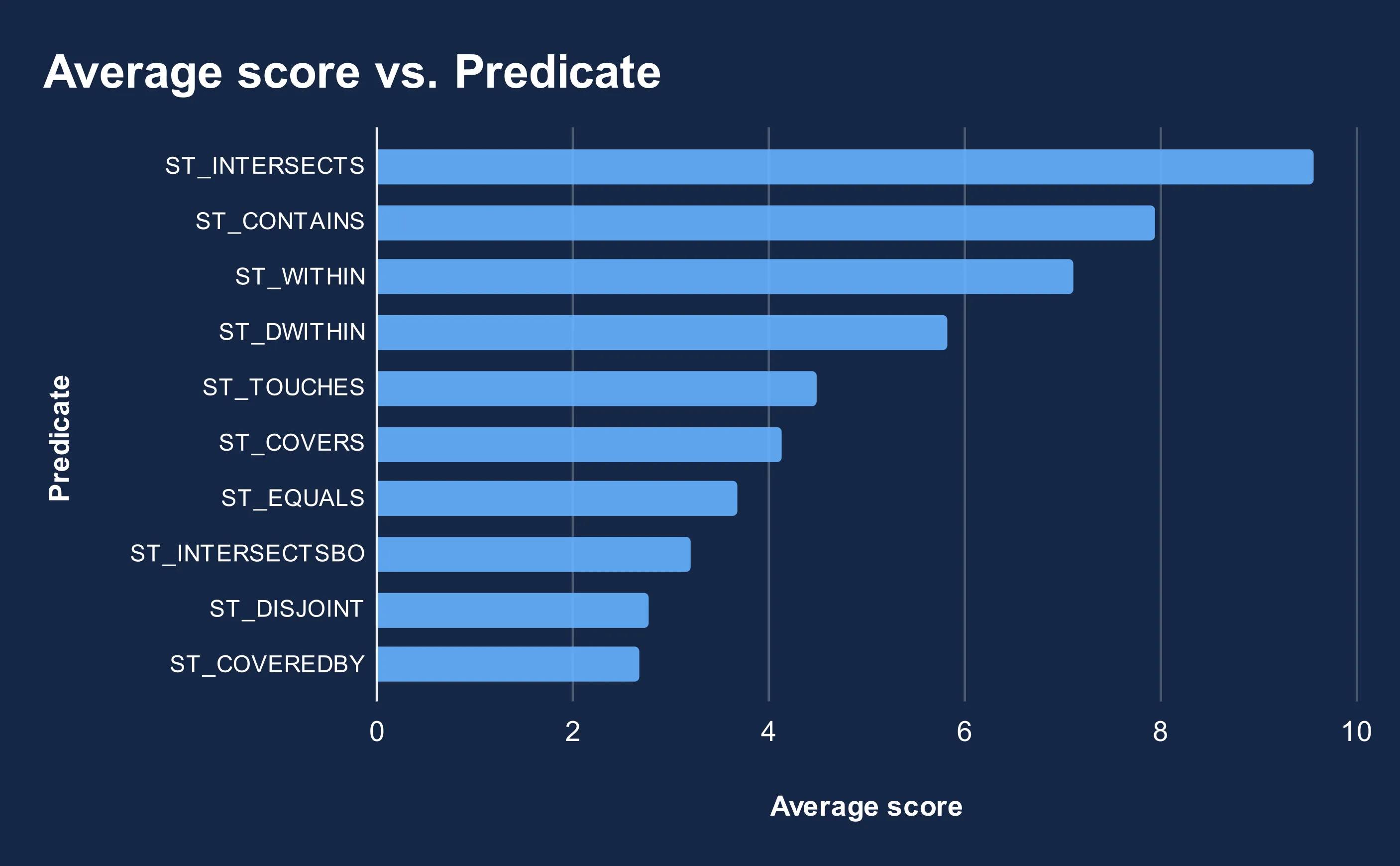
Our survey says…
There are multiple types of spatial predicate and to help shape this article we wanted to hear from YOU which are the most popular! We ran a poll across Twitter and LinkedIn asking our followers to rank 10 of the most common Spatial Predicates by how frequently they use them with 10 being the most frequent use. The results are in and our winner is… ST_INTERSECTS!
Keep reading as we run through what these are and how when and why to use them!
Before we start…
You’ll see a running theme in this guide: the results of a Spatial Join are only as good as the geometry of the data. Imprecise and inaccurate geometries - such as overlaps or slither gaps - can cause erroneous results. For this reason it’s always important to carefully inspect your source data as well as the results of any join for accuracy. Throughout this post we’ll share our top #ProCARTOtips for dealing with these issues! 👀 👀
In the maps below we’ll be using Broomfield County Colorado (from Tiger/Line geographic data from the U.S. Census Bureau) to filter a H3 hexagon grid (made available through CARTO’s Spatial Features layers) to illustrate various spatial predicate concepts. You can subscribe to both of these datasets via our Spatial Data Catalog.
#1: ST_INTERSECTS
The clear winner ST_INTERSECTS returns a “true” result if any part of the join feature touches or overlaps with any part of the target feature including their boundaries.
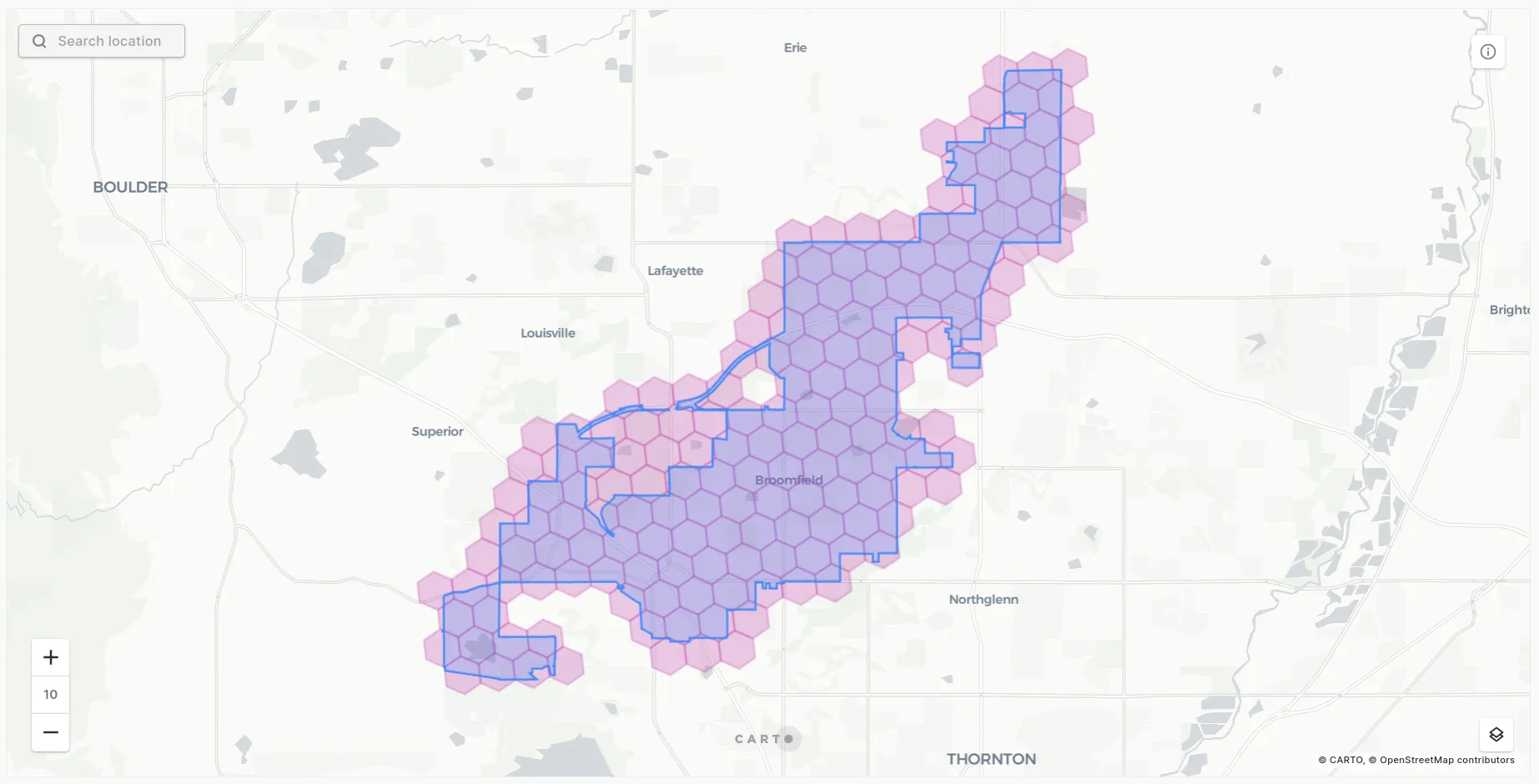
WITH aoi AS (SELECT * FROM carto-data.ac_lqe3zwgu.sub_usa_tiger_geography_usa_county_2018where do_label like ‘%Broomfield%’)
h3 AS (SELECT * FROM carto-data.ac_lqe3zwgu.sub_carto_derived_spatialfeatures_usa_h3res8_v1_yearly_v2)
SELECT h3.geoid AS h3 FROM h3  aoi
WHERE ST_INTERSECTS(aoi.geom  carto-un.carto.H3_BOUNDARY(h3.geoid))
ST_INTERSECTS is best employed for use cases where it doesn’t matter if features fall wholly inside each other or not. Examples could include:
- How many counties does a highway pass through?
- Which buildings are impacted by a flood event?
- How many vehicles are currently in my operating area?
Note: don’t confuse this with ST_INTERSECTION! This is a transformation function (rather than a predicate) which means it returns the geometry of the intersecting area and doesn’t work as a predicate.
Enriching data - area-based intersection
#ProCARTOtip A really useful type of Spatial Join is an area-based join. Often (actually typically!) different geospatial layers won’t neatly line up and that can make intersections a challenge and so joins need to be performed based on the percentage of intersecting area.
For example take the map above. Say we want to extract the population from the output areas (blue lines) to understand the total population within our study area (the pink area) - the challenge here is these don’t exactly line up. To get as accurate a figure as possible we’d need to allocate the population by the % of the output area which falls within the study area. So for instance if 50% of an output area lies inside the study area then 50% of the population would be allocated.
Performing this sort of analysis with SQL can actually be quite complex and the code quite extensive - both of which open up the potential for human error. We’ve created a series of enrichment tools to streamline this process for our users. Our tools perform area-based intersections (or length-based for line features) so our users can quickly and easily aggregate their data - check out the code below to see how simple this is!
CALL carto-un.carto.ENRICH_POLYGONS(
  R’’’
  SELECT * FROM targetdata
  ’’’
  ‘geom’
  R’’’
  SELECT * FROM joindata
  ’’’
  ‘geom’
  [(‘joinvariable1’  ‘aggregatecalculation’)  (‘joinvariable2’  ‘aggregatecalculation’)…]
  [’my-project.my-dataset.my-enriched-table’]
);
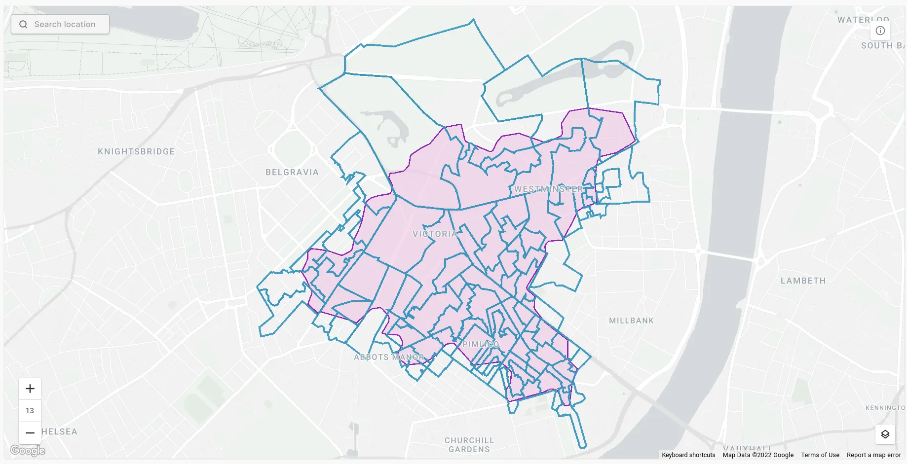
This means you can really easily and quickly visualizations like the below in just a few lines of code! This visualization shows levels of car ownership in London using H3 cells which have been enriched from the census zone source data (output areas).
Check out our full guide to data enrichment here!
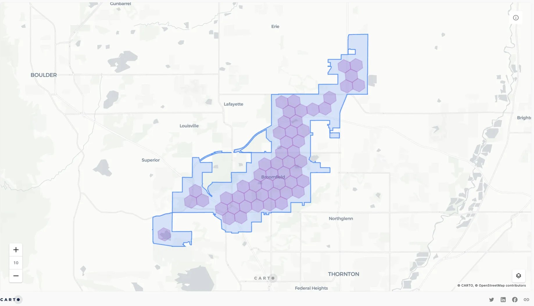
#2 & #3 ST_CONTAINS & ST_WITHIN
In second and third place respectively are ST_CONTAINS and ST_WITHIN. It’s no coincidence that these two ended up so close together; they’re essentially two sides of the same coin.
ST_CONTAINS will return “true” where the target feature contains all parts of the join feature but do NOT touch their boundary. ST_WITHIN is the reverse so ST_CONTAINS(geometryA geometryB) will return the same thing as ST_WITHIN(geometryB geometryA).
You can see the results of this illustrated below.
#ProCARTOtip A common use case of spatial joins is in understanding the relationships between different zones in a hierarchy; for instance which census tracts fall within which county. If your zone data comes from different sources there may be slight discrepancies between the geometries of the two layers. These can play havoc with your spatial predicates. If you’re having issues with this try using ST_CENTROID(joindata.geometry) to convert your join layer to points then run ST_CONTAINS.
#4 ST_DWITHIN
If you work in transport or logistics ST_DWITHIN will be your spatial predicate go-to! The “D” here stands for “distance;” this predicate returns “true” for target features within a set distance of your join feature (including features which intersect the target feature). The syntax is a little different for this one:
…ST_DWITHIN(targetdata.geometry joindata.geometry distancethreshold)
The applications for this are huge! They could include:
- Counting the number of competitors within a radius of your store
- Finding the total population within a radius of a new EV charging station
- Understanding the skills market or unemployment levels around a new distribution center location
#5 ST_TOUCHES
Coming in at number 5 it’s ST_TOUCHES! This predicate is basically the opposite of ST_CONTAINS. It returns “true” where the join feature touches the boundary of the target feature but not the interior.
ST_TOUCHES is really useful for finding neighboring zones for example if conducting forms of slope analysis. It’s also something you’ll probably make more use of when working with linear data. In particular ST_TOUCHES is useful for network analysis where the topology (i.e. how features connect) is crucial.
#6-10
Now to round up our bottom 5!
- #6 ST_COVERS is similar to ST_CONTAINS with the difference being that the boundaries of the two features may be touching to return a “true” result. This predicate returns “true” when the target feature covers the entirety of the join feature including the join feature’s boundary.
- #7 ST_EQUALS tests whether two features are spatially identical. This is super useful for evaluating the quality of data or assessing two sources against each other.
- #8 ST_INTERSECTSBOX tests the geometries against the target feature’s bounding box (i.e. a box that covers the extent of each feature with bordering lines which run parallel to lines of latitude and longitude).
- #9 ST_DISJOINT is the opposite to our winner ST_INTERSECTS! This predicate returns “true” where no part of the join feature touches the target feature including their boundaries.
- #10 ST_COVEREDBY comes in at a humble 10th place. ST_COVEREDBY is the reverse to ST_COVERS returning “true” if the join feature covers the entirety of the target feature including its boundaries.
This ranking is the result of an entirely democratic vote from the people who happened to see our social media posts about this however the way you use Spatial Predicates Joins and Filters will be entirely dependent on your use case.
Spatial Joins for Location Intelligence
While it may not have been the most glamorous awards show we hope you found our run-down of Spatial Joins Filters and Predicates useful! Want to learn more? Check out some more of our SQL guides and tutorials here.