How to Enrich POS Data to Analyze & Predict CPG Sales

Over the past year consumer behavior has changed significantly and many believe permanently. Last year U.S. CPG sales rose by 10.3% to $933 billion as consumers stocked up on pantry items  cleaning products  and other consumer goods.

   {% include icons/icon-quotes.svg %}    Consumer habits  once they're established in our categories  are rarely reversed. We do expect that there's some stickiness to new habits that are being formed.
       Jon Moeller  COO & CFO at Procter & Gamble.    

Even though the market grew  large manufacturers lost 1.3% in market share  or $12.1 billion in sales  to smaller players fulfilling the supply shortage in categories including soap  hand sanitizers  and home health care kits.

It’s clear that there are many opportunities for players of all sizes within the CPG industry with many analysts now focused on precisely where  in a geographical sense  to focus their efforts. As we have looked at in previous posts  the use of Spatial Data Science not only allows a deeper understanding of historical sales performance but can also be used to predict future growth in new markets and territories.

In this case study  we propose an approach to leverage multiple types of spatial data in order to analyze the factors that impact point-of-sale (POS) performance. Usually  this would involve time series analysis per region or per outlet/merchant  where the sales of each stock-keeping unit (SKU) are modelled at a weekly level. Herein  a different approach is presented where the spatial variability is studied in order to identify the driving factors that result in different sales performance across regions.

As a first step  we leverage CARTO's Spatial Features dataset to build a model that analyzes sales performance taking into account the volume and type of Point of Interest (POI) in the vicinity of each merchant. As a second step  we complement the POI-based features with other spatial datasets available via the Data Observatory to further improve the inference. In order to illustrate and compare the improvement that the additional spatial signals offer to the prediction  two models for each SKU are built: one that uses only the POI counts and a second one with the additional drivers from the other datasets. In both models  the area of interest (AOI) is split in cells  using an H3 grid with resolution 6  and the sales are aggregated as the weekly average for the period 2018-2019.

Data Sources

For the purpose of this analysis  the publicly available Iowa Liquor sales data were used. This dataset contains spirits sales information at Iowa Class "E" liquor licensees by product and date of purchase from January 1  2012 to current. Class "E" license is described as:

For grocery  liquor and convenience stores  etc. Allows for the sale of alcoholic liquor for off-premises consumption in original unopened containers. No sales by the drink. Sunday sales are included. Also allows wholesale sales to on-premises Class A  B  C and D liquor licensees but must have a TTB Federal Wholesale Basic Permit.

The sales data points were aggregated at weekly level for each product and store. By product  it is considered the concatenation of the item description and the bottle size.

In order to analyze the sales variation across the different locations within the state of Iowa  we selected different spatial data sources available in CARTO's Data Observatory that could help us identify which factors affect the sales of SKUs in that state.

As mentioned in the introduction  the first model is built leveraging:

• CARTO Spatial Features: population  age  and gender  and points of interest counts across different categories.

Then  in the second model we include additional features from the following datasets:

• Geographic Insights from Mastercard : providing sales-based dynamics of a location with indices measuring the evolution of credit card spend  number of transactions  average tickets  etc.  happening in a retail area over time;
• Geosocial Segments from Spatial.ai: behavioral segments based on the analysing social media feeds with location information;
• Sociodemographics from AGS: basic socio-demographic and socio-economic attributes estimated at current year;
• Human Mobility - Patterns from Safegraph:visits attribution to points of interest over time;
• Bigquery Public Datasets - Census Bureau US Boundaries.

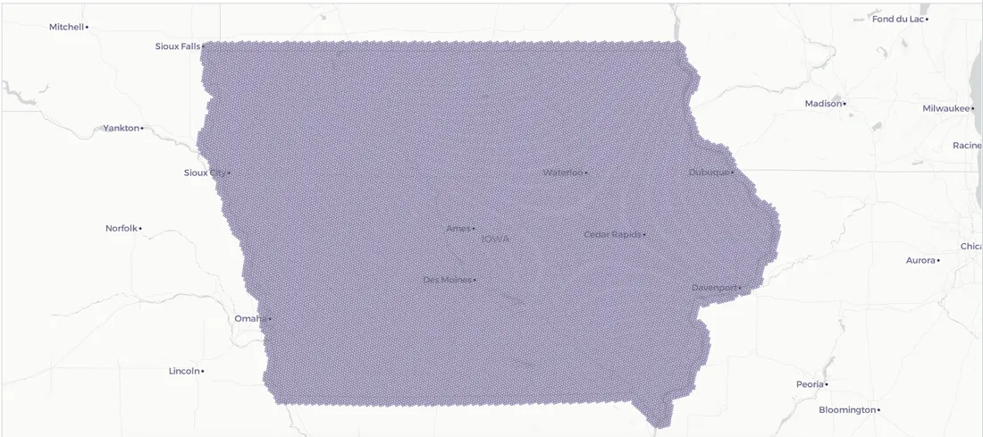
The state of Iowa was split into hexagonal grid cells with resolution 6 using the standard format of an H3 grid  which resulted in 4 428 cells with each cell covering circa 65 sqKm. The rationale for this was to examine the drivers over an area and not on specific merchant locations. The specific resolution was selected as a good candidate  being granular enough to introduce variability and wide enough to capture the effects of an area. The resulting grid is shown in the following figure:

We focused our analysis on the following three SKUs:

• Hawkeye_vodka_1750
• Titos_handmade_vodka_1000
• Captain_morgan_spiced_rum_1000

For each of these SKUs  the average weekly sales per H3 cell was calculated. The period 2018-2019 was used  as in 2020 the sales were not stable as a lot of stores closed or underperformed due to the impact of Covid-19. In addition  the average weekly sales were scaled by the number of stores in each cell  in order to capture the average performance per store within an area. Finally  the sales were scaled by the population  hence creating an index per cell signaling the preference of the particular SKU. The log of this signaling value will be modelled at the end. The rationale of these transformations is not only to create an index  but also to normalize the variable to be modeled.

An example of the signal for SKU "Vodka Hawkeye 1750 ml" can be seen below:

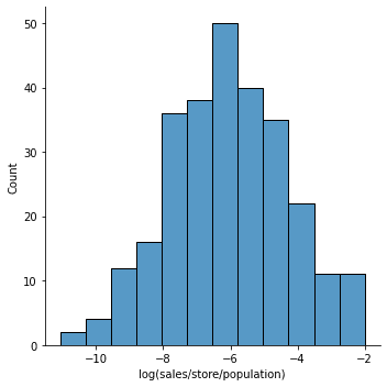
These transformations enable us to perform sales predictions in other areas or states without knowing the number of stores per cell  thus getting insights on the market potential of this type of product in other areas for which we do not have actual sales data (as we will show later on in this post).

Please note that this analysis was performed per SKU but in some cases it can also be performed by brand  manufacturer etc. depending on the level of analysis the user wants to perform.

Data Enrichment

Each cell of the grid was then enriched with the following features using the Data Enrichment methods available in CARTOframes.

For the first model we used:

• CARTO Spatial Features: Male/Female population  POIs related with transportation  leisure  healthcare  food & drink  financial  education  retail  tourism.

Then  in the second model we enriched the following features:

• Mastercard Geographic Insights: Average ticket transaction for Total Retail category;
• AGS Sociodemographics: Average income  Medium Age;
• AGS Consumer Spending: Average household spend in alcoholic beverages;
• Spatial.ai Geosocial Segments: whiskey business  wine lovers  late night leisure  party life  hip hop culture;
• Safegraph Patterns: Average number of visits per week in each cell  average distance travelled from home.
• Census Bureau US Boundaries: For each cell the percentage of area that is considered as urban was calculated.

An example of the resulting features can be seen in the following map:

For each of the selected variables in the Data Enrichment phase  spatial lagged values based on the neighboring cells were calculated. We computed two types of lagged values  one for the sum of the neighboring values and one for the average value across neighbors. Note that neighboring cells are considered to be ones that share an edge with the cell of interest. For the features such as population  points of interests  and number of visitors  the sum was used  while for the rest the average value was considered. For example  in the diagram below  the sum lagged value is 62 while the average value is 10.3:

Feature selection

For the feature selection analysis we only use the cells with actual SKU sales  discounting those with no sales since the dataset only contains certain stores.

Before proceeding to the feature selection process  the features first need to be transformed. The POIs  along with their lagged values  were Min-Max scaled while the rest of the variables were standardized. Min-Max was selected for the POIs as these are integer numbers showing the quantity of each category in an area and with Min-Max an index is created showing how fulfilled each area is with respect to the rest. Scaling of features is a common practice as if it is not applied then the features with the highest magnitude tend to dominate. Thus  with this process everything is brought to the same reference.

The feature selection process refers to the second model  where the additional features apart from the Spatial Features POIs are used.

The first step in feature selection is to remove correlated features and this was done by using the Variance Inflation Factor(VIF). For every SKU  the process of feature selection has to be repeated as the relevant cells are different in each case. The process with VIF is the following:

1. Compute VIF for each variable
2. Sort them in descending order
3. Remove the highest if greater than 20  if not exit
4. Go back to step 1

In that way  we ensure no major multicollinearity amongst the remaining features. Following the previous selection; for each SKU  a backward selection process using Linear Regression took place  removing a covariate with p-value greater than 0.1. After the removal  the modeling runs from scratch. An example of the process and the remaining features for the SKU ‘vodka_hawkeye_1750' can be seen below:

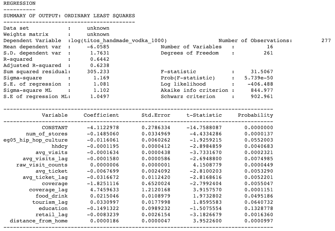
Below is a table detailing the variable abbreviations and descriptions. The {variable's name}+"_lag" variable indicates the lagged version of the variable.

Spatial Modeling

Having reduced the dimension of the explored features  we proceed to build the spatial model.

Methodology

As described in the introduction  two types of spatial models were generated:

1. Only using the POIs from the Spatial features;
2. Using all the resulting features from the previous feature selection procedure and leveraging all introduced spatial datasets.

For each model  a Stacked Ensemble algorithm was built for the final regression.

For each SKU  using a K-fold with 5 folds on the dataset  5 different models were trained  each one of them for a different training set. The model was based on Kinging Regression using the Random Forest algorithm as a base. Each model was validated for the remaining part of the dataset  and the R-squared (R2) on the validation was saved as a weight weight_j_sku  where j is the number of the model and sku the target SKU.

In the end  for each SKU  5 different models were trained. For the inference  the prediction was calculated as:

Where y[s] is the prediction of the sku at cell s  

the j^th model for SKU  and weight:

Results

In the table below  the R-squared and the mean absolute error (MAE) for each SKU and model (only Spatial Features POIs and all other features) can be seen. Please note that the errors refer to average weekly sales per store  meaning that the error of the model was scaled back by the population. As a reminder the modelled variable had been normalized by the population of each cell. The model with just the Spatial Features POIs performed only slightly worse than the model with the full features  demonstrating the strong modeling capabilities of the Spatial Features dataset.

One very important observation is that the SKU with 1000ml bottle size performed better than the 1750ml SKUs. One possible explanation is that the larger volume products may refer more to businesses rather than to home/individual consumption. Thus  in one future analysis we should treat the larger volume products differently than the rest  as these could consist of sales from wholesalers to businesses (which pose different commercial dynamics than small retailers selling to individuals).

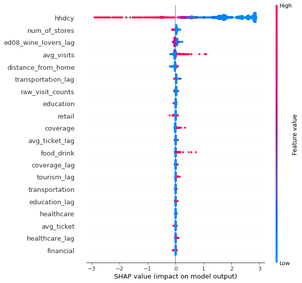
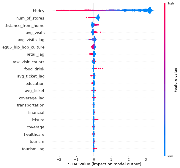
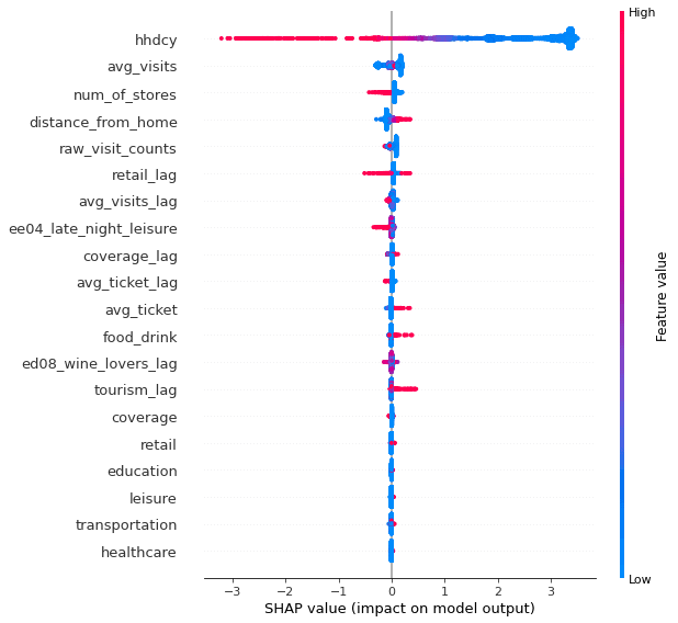
For each SKU the Shapley values of one model from the ensemble can be found below. It is observed that the most significant factors are the number of households per cell  the average number of visits to POIs in that cell from Safegraph dataset  and the food & drink POIs from Spatial Features. For all three SKUs  the number visits to POIs is an important factor with positive impact  as you expect that foot-traffic can be translated to an indicator of the purchase power of an area. In addition  the lagged version of some variables such as the number of POIs in retail and tourism categories  which indicate what happens in the adjacent cells  also seems to be important to model point of sales performance. The number of POI in the adjacent cells tends to affect the vicinity area either in a positive or negative way. For example  with Hawkeye vodka  the tourism lag variable has a positive correlation with the sales  meaning that the larger number of touristic POIs in the vicinity translates to higher sales.

Hawkeye_vodka_1750

SHAP values for SKU Hawkeye_vodka_1750Titos_handmade_vodka_1000

SHAP values for SKU Titos_handmade_vodka_1000Captain_morgan_spiced_rum_1000

SHAP values for SKU Captian_morgan_spiced_rum_1000

Using the model to estimate sales potential in a different region

Using the second model built in the previous section  we can derive an estimation of the sales potential of the three SKUs in the state of Nebraska  an area which we do not have actual point of sales data. The state of Nebraska was also split in an H3 grid with the same resolution as in Iowa  and the cells were enriched with the information described in the previous section on Data Enrichment. Then  for each of the three SKUs  the spatial model with all the selected features was applied and the output is illustrated below. In the context of a CPG product roll-out strategy or for Site Planning in Retail  this step is useful to craft the go-to-market strategy when entering into a new territory for which you still do not have any performance indicator. Deep diving into the figures  the highest values are observed close to the main cities of Nebraska and very low values in the areas which seem to be isolated  as it would be expected.

Sales prediction for SKU Hawkeye_vodka_1750

Sales prediction for Titos_handmade_vodka_1000

Sales prediction for SKU Captian_morgan_spiced_rum_1000

Conclusions

Available Iowa Liquor data were analysed from a spatial perspective  aiming to reveal the factors that drive the consumption of the different SKUs and the variation across different areas within the state of Iowa. The analysis was performed at SKU level and the period 2018-2019 was used. The state was split into a grid of H3 cells at resolution 6 and each cell was enriched with data from the Data Observatory (i.e.  demographics  financial  human mobility  behavioral  and points of interest).

We presented a methodology to select the most relevant features and how to model the average weekly sales leveraging Spatial Data Science. In the end  we extrapolated the results for the state of Nebraska  for which we do not have sales data  in order to identify those areas with more potential to sell those SKUs.

Want to get started?

Sign up for a free account

This project has received funding from the European Union's Horizon 2020 research and innovation programme under grant agreement No 960401.