Aggregating data for faster map tiles


We have recently implemented dynamic aggregation for both raster and Mapbox Vector Tiles in CARTO's Engine.You can find the documentation here.
Engine is the platform that powers CARTO Builder and allows developers to create Location Intelligence apps; one of its services the Maps API provides map tiles so that the results of analyses performed with CARTO can be represented in online maps.
With our new dynamic aggregation capabilities we try to ease the problem of representing too many points in a map. Visualization of point data in maps breaks down when the feature density is too high; on one hand processing many individual point records is time consuming and on the other hand we'll end up with symbols at the same spot obscuring one another.
We can handle this case by aggregating the points spatially so that points lying close to each other are grouped into a single entity which summarizes the data for the whole group.
The idea isn't new and has been in use by CARTO's torque maps for a long time as well as by the overviews feature.
Basically we're trading some additional backend processing time (to perform the aggregation) for lighter data transfers and less features to be rendered.
For example here's the average tile generation & transfer time for a 8-tile map containing 258K points.
{:.tb__content}
| Tile type | No aggregation | Default aggregation | Speed up |
|---|---|---|---|
| PNG | 5.0 s | 1.4 s | 3.6x |
| MVT | 3.4 s | 1.1 s | 3.0x |
Here the MVT average size has been decreased from 10.4MB to 2.4MB.
How It works
We use a simple grid aligned with the tile we're generating to cluster points spatially and replace each cluster (the points lying inside the same grid cell) with a single point summarizing its group. By default the aggregation cell size corresponds to the on-screen pixels size so that the visual impact of the aggregation is minimal.
Now how should we summarize multiple points (with their data attributes) into a single one?. The answer to this depends on the nature of the attributes as well as on the intended visualization. If we have a temperature attribute it could be convenient to have the average value at each aggregated point; but if the original temperature was a maximum then computing maximum values might make more sense.
So we introduced a mechanism in map instantiation that allows users to specify how they want their data aggregated; the aggregation columns parameter defineswhich aggregated columns are computed and placement specifies where the resulting point is placed. An additional _cdb_feature_count attribute is always present denoting the number of original records grouped for each result record.
Default aggregation (sampling)
But there's a particular use case for aggregation for which requiring users to specify the details is not appropriate: existing visualizations that don's specify any aggregation parameters can benefit from automatic aggregation when the number of points is so large that the original visualization would just break down (due to timeout limits) or would be too slow. In this case the aggregated data should be apt for the original visualization based on the un-aggregated original data. This requires that all the original attributes are present and that some basic properties are preserved (e.g. if a numeric value represents a category averaging such values would introduce invalid results).
To support this case the aggregation works differently when no explicit aggregation parameters are provided(more precisely: when no parameters that define the aggregated result attributes placement or columns are present).
In this case for each spatial cluster we pick a random member (ok not so random the one with the lowest cartodb_id value) to represent the group.So we are effectively sampling the data spatially. Working with a sample of the data allows any processing/styling intended for the original data to be valid.This is not a perfect solution since some visualizations (e.g. involving spatial densities) won't be strictly correct but it's a good compromise that will make most maps work with larger datasets without any adjustment. For more precise results users must handle large datasets differently from smaller ones and plan their visualizations with aggregation in mind.
How to use it
The aggregation details are determined for each layer when a map is instantiated. A map is instantiated by sending the map configuration (MapConfig)to the proper API endpoint like this:
{% highlight javascript %}const mapConfig = { … };const response = await fetch(URL_BASE + '/api/v1/map' { method: 'POST' headers: { 'Accept': 'application/json' 'Content-Type': 'application/json' } body: JSON.stringify(mapConfig) });const layergroup = await response.json();{% endhighlight %}
A minimal MapConfig with explicit aggregation options would look like this:
Multiple layers can be contained in a single vector tile or rendered into a raster tile but each layer can have individual aggregation options.
{% highlight javascript %}{ layers: [ { options: { sql: 'select * from TABLE' aggregation: { … } } } ]}{% endhighlight %}
For raster maps the MapConfig must also include CartoCSS styles:
{% highlight javascript %}{ layers: [ { options: { sql: 'select * from TABLE' aggregation: { … } cartocss: ... cartocss_version: '3.0.12' } } ]}{% endhighlight %}
Not all datasets benefit from aggregation; for a moderate number of features there's no need for aggregation. And only point geometries aggregation is supported at the moment. So aggregation may or may not be performed by default and even if the user explicitly defines aggregation options there's a minimum threshold for it to be applied.
We provide the information on whether a layer will be aggregated or not (and for which tile formats it will) in the map instantiation response(layergroup in the previous example);
note the metadata.layers[0].meta.aggregation property here
{% highlight javascript %}{ "layergroupid": "7b97b6e76590fef889b63edd2efb1c79:1513608333045" "metadata": { "layers": [ { "type": "mapnik" "id": "layer0" "meta": { "stats": { "estimatedFeatureCount": 6232136 } "aggregation": { "png": true "mvt": true } } } ] } }{% endhighlight %}
The response also includes some properties ommitted here that ara useful for using the map tiles in various mapping libraries:
- layergroup.metadata.tilejson (see TileJSON spec) useful for Mapbox GL or OpenLayers.
- layergroup.metadata.url url template useful for libraries like LeafLet.
Aggregation parameter details
The available aggregation parameters for layer are placement and columns which define the aggregated attributes in the result resolution and threshold that define how and when to aggregate.
placement
Determines the kind of aggregated geometry generated; the possible values are point-sample point-grid and centroid.
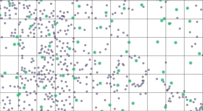
point-sample
This is the default placement. It will place the aggregated point at a random sample of the grouped points like the default aggregation does. No other attribute is sampled though the point will contain only the aggregated attributes determined by the columns parameterand the _cdb_feature_count.
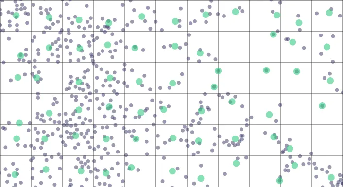
Example: here the smaller dots are the original data points; the greenish bigger dots are the aggregated points and the lines show the aggregation grid.
point-grid
Generates points at the center of the aggregation grid cells (squares).
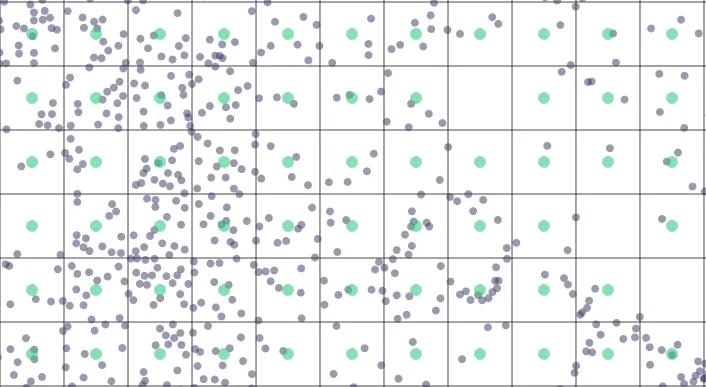
centroid
Generates points with the averaged coordinated of the grouped points (i.e. the points inside each grid cell).
columns
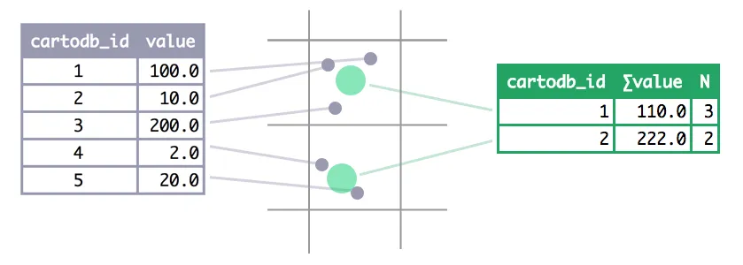
The aggregated attributes defined by columns are computed by a applying an aggregate function to all the points in each group.Valid aggregate functions are sum avg (average) min (minimum) max (maximum) and mode (the most frequent value in the group).The values to be aggregated are defined by the aggregated column of the source data. The column keys define the name of the resulting column in the aggregated dataset.
For example here we define three aggregate attributes named total max_price and price which are all computed using the same column price of the original dataset but applying three different aggregate functions to it.
You can use the original column names as names of the result but all the result column names must be unique. In particular the names cartodb_id the_geom the_geom_webmercator and _cdb_feature_count cannot be used for aggregated columns as they correspond to columns always present in the result.
{% highlight javascript %}{ "columns": { "total": { "aggregate_function": "sum" "aggregated_column": "price" } "max_price": { "aggregate_function": "max" "aggregated_column": "price" } "price": { "aggregate_function": "avg" "aggregated_column": "price" } } }{% endhighlight %}
This is independent of the number of pixels for raster tile or the coordinate resolution (mvt_extent) of vector tiles.
Note also that even though the resolution parameter takes on the torque convention ofdividing by default each tile into 256x256 cell units (corresponding to the resolution value 1) there's nothing special about such value and you can use both any aggregation cell size.
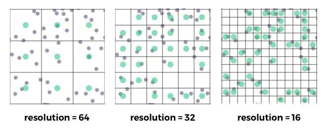
resolution
Defines the cell-size of the spatial aggregation grid. This is equivalent to the CartoCSS -torque-resolution property of Torque maps.
The aggregation cells are resolution×resolution pixels in size where pixels here are defined to be 1/256 of the (linear) size of a tile.The default value is 1 so that aggregation coincides with raster pixels. A value of 2 would make each cell to be 4 (2×2) pixels and a value of0.5 would yield 4 cells per pixel. In general values less than 1 produce sub-pixel precision.
threshold
This is the minimum number of (estimated) rows in the dataset (query results) for aggregation to be applied. If the number of rows estimate is less than the threshold aggregation will be disabled for the layer; the instantiation response will reflect that and tiles will be generated without aggregation.
About the buffer size:
For vector tiles it may be important to define the buffersize parameter appropriately.
This parameter defines a distance around the tile. Features that lie within this distance of the tile will be included in the resulting MVT.
Just like for raster tiles This may be required for labeling the features correctly but in the case of vector tiles the features will be present in the result so they will be duplicated for neighbouring tiles; to avoid the overhead of unnecessary processing in the client the buffer size should be as small as possible.
For raster tiles the buffersize can be defined in the CartoCSS but for vector tiles it should be defined through the MapConfig buffersize parameter which allows to define different values for each tile format:
{% highlight javascript %} buffersize: { 'png': 0 'grid.json': 64 'mvt': 0 } {% endhighlight %}
Both for vector and raster tiles If the aggregation cell size (as determined by the resolution) is less than the buffer size unexpected results may appear; in general we recommend using a buffer size of 0 when aggregating data.