Calculating Catchment Areas with Human Mobility Data
Catchment areas (i.e. trade areas) are the geographic areas from which retailers wholesalers and other commercial locations draw most of their business. Calculating them properly is essential in sectors such as Retail and Real Estate as they allow organizations to better understand customers and develop appropriate business strategies.

There are numerous techniques to calculate catchment areas from circular trade areas through isochrones gravitational models to more sophisticated techniques that incorporate location specific variables. The technique chosen often depends on the information and data available and the available expertise in the different techniques.
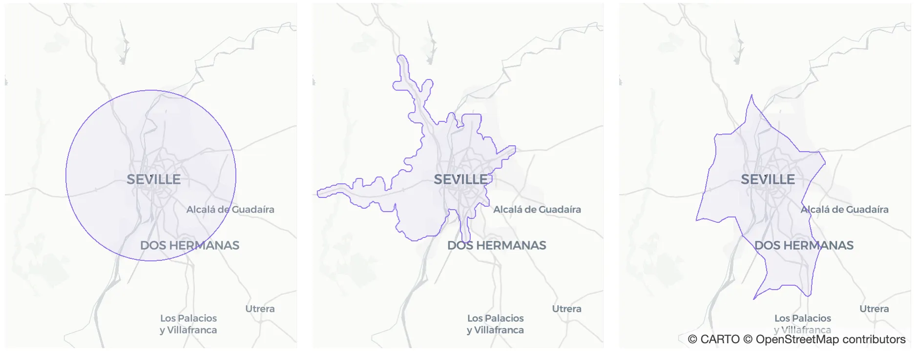
Fig 1. Different catchment areas depending on the technique: Circular trade area (15 km buffer) on the left 20-minute by car isochrone in the middle and catchment area based on mobility data on the right.
When a new store is opened the lack of available data makes it very difficult to know what customers will come to that store or where they will come from. In the absence of this data the most common approach is to calculate buffers or isochrones around the target location but this approach lacks precision and can lead to unreliable findings.
For example taking the same time-isochrone for two locations regardless of the population density around them will most certainly lead to unreliable findings. This is because people who live in low density areas normally travel longer distances to do shopping than people who live in high density areas. Here we aim at calculating reliable potential catchment areas using human mobility data as a proxy of the potential customers.
The results obtained show that traditional approaches like isochrones or buffers fail to capture where people visiting a specific location actually come from. They don’t provide the flexibility to build targeted catchment areas in the way that the use of human mobility data does; being able to compute for example different catchment areas for weekday and weekend visitors.
Human Mobility Data
The base of our method is the use of human mobility data from Vodafone Analytics. This data provides insights on the number of people visiting any 250m x 250m grid cell covering the entire territory of study. Vodafone anonymizes aggregates and then extrapolates the data measured in the network to provide insights representing the overall national and international population.
In addition this data provides the origins of the visitors aggregated at different levels depending on the distance to the destination cell. For visitors coming from the same municipality the origins are provided also at the 250m x 250m cell level; for visitors coming from other municipalities within the same province visits are aggregated at the municipality level; and for visitors coming from other provinces visits are aggregated at the province level. Although it is also provided given the characteristics of this study we are not going to consider the origins of visitors coming from different countries.
In addition this data can be disaggregated by type of activity at origin (home/work) day of the week and time of the day (morning/afternoon/evening). The data can also be disaggregated by sociodemographic variables: age range gender and economic status.
For the purposes of this use case we selected a target location in the city of Sevilla in Spain to show the methodology. On the map below the origins from where visitors come from are shown.
Fig 2. This choropleth map shows number of visitors by origin normalized by the total population at that origin.
We also use demographic data from Unica360 another of our data partners to normalize visitor data. Unica360’s data is provided aggregated in a 100m x 100m cell grid and includes among other variables population population by age range and number of households. The data aggregation is upscaled to fit Vodafone’s 250m x 250m cell grid applying areal interpolation.
Defining our Approach to Catchment
The first idea for calculating the catchment areas was to compute for every origin-destination pair an index measuring the destination’s visitor attraction potential with respect to that origin. Here the destination is understood as the grid cell containing the location for the new store.
The index would be defined as:
$$I_{ij} = f(n_{ij} d_{ij}); \forall i j$$
where
- $$n_{ij}%0$$ is the number of visitors at destination j coming from origin i
- $$d_{ij}%0$$ is the distance from origin i’s centroid to destination j’s centroid
- $$f:\mathbb{R}^2 \rightarrow\mathbb{R}%0$$ is the index function
Based on this index we would calculate every destination cell’s catchment area by selecting the origins with the highest index value that made up 70% of the total visits at that destination cell.
However since the number of visitors coming from other municipalities and provinces is not available at the cell level this first idea needs to be adapted with a new approach that allows one to compare the number of visitors at different aggregation levels (cell municipality and province).
This new approach has two main steps:
- Finding the minimal isochrone (based on travel time by car) covering the origins of at least 80% of the destination cell’s visitors.
- Reducing the size of the catchment area by selecting among the previous origins those with the highest index value that make up 70% of the total visitors to that destination cell.
Finding the Minimal isochrone
As mentioned before visitors coming from other municipalities in the same province and from other provinces are aggregated at the municipality and province level respectively. Isochrones allow us to consider only those areas within a municipality/province which are closer (in time) to the destination cell. The method developed calculates increasingly larger isochrones until 80% of the destination cell’s total visitors are covered.
In order to calculate the number of visitors coming from the intersection of an isochrone with a province (or municipality) $$nvisitorsIntersection%0$$ the next steps are followed:
- First the proportion of the province’s population living in the intersection is calculated using the demographics data at 250x250m grid cells $$pctPopulationIntersection%0$$
- Secondly the number of visitors coming from the intersection is calculated with the formula below. This formula is based on Tobler’s law of geography and the use of empirical data to find a rough fit.
$$nvisitorsIntersection = nvisitorsProvince \cdot \sqrt[2.5]{pctPopulationIntersection}%0$$
The function $$\sqrt[2.5]{-}%0$$ assigns more visitors as coming from areas within the province that are closer to the destination cell (and hence fewer to areas further away). In the figure below it can be seen how this function will assign 70% of the visitors coming from a province/municipality to an area containing only 40% of the population but that is closer to the destination cell. Again we are applying this formula based on the assumption that people living closer to the destination cell are more likely to visit it. More sophisticated models could give better predictions.
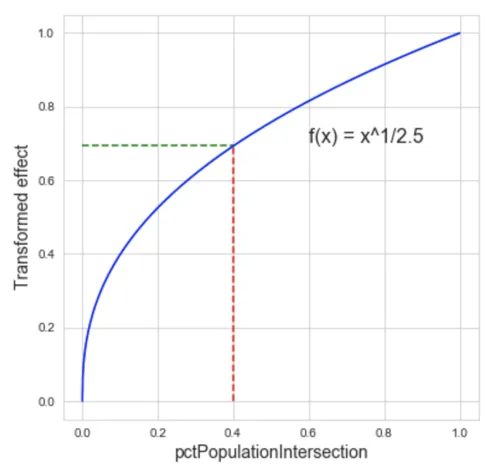
Fig 3. Transformation function to assign more visitors to closer places.
Selection of Visitor Origins
Once we have the minimal isochrone the next step is to calculate the index value of each origin within the minimal isochrone which is defined as follows:
$$I_{ij} = \dfrac{n_{ij} }{d_{ij} }; \forall i j%0$$
This index is calculated using the normalized number of visitors coming from each origin $$norm_nvisitorsIntersection%0$$. The normalization is done by dividing by the number of population cells within the intersection $$npopcellsIntersection%0$$ i.e. the number of visitors is distributed uniformly among all population cells within the intersection polygon.
$$norm_nvisitorsIntersection = \dfrac{nvisitorsIntersection}{npopcellsIntersection} %0$$
This normalization allows the comparison of visitors coming from cells within the same municipality with visitors coming from other municipalities and provinces.By selecting the origins with the highest index values that make up 70% of the destination cell’s total visitors we get its estimated catchment area.
Process and Visualizing the Results
The following figure shows the three iterations needed to calculate the minimal isochrone containing at least 80% of the total visitors of a destination cell in the city of Sevilla.

Fig 4. This visualization shows the three iterations needed to get to 80% of a cell’s total visitors. The color shows the value of the index defined as a function of the normalized visits and the distances between centroids.
Once the minimal isochrone is found and the index is calculated for every origin we can build the catchment area. Finally the concave hull (aka alpha shape) of the catchment area is calculated in order to have manageable connected areas. For calculating the convex hull we used the Python library alphashape.
The figure below shows the raw catchment area for the destination cell in Sevilla and its concave hull.
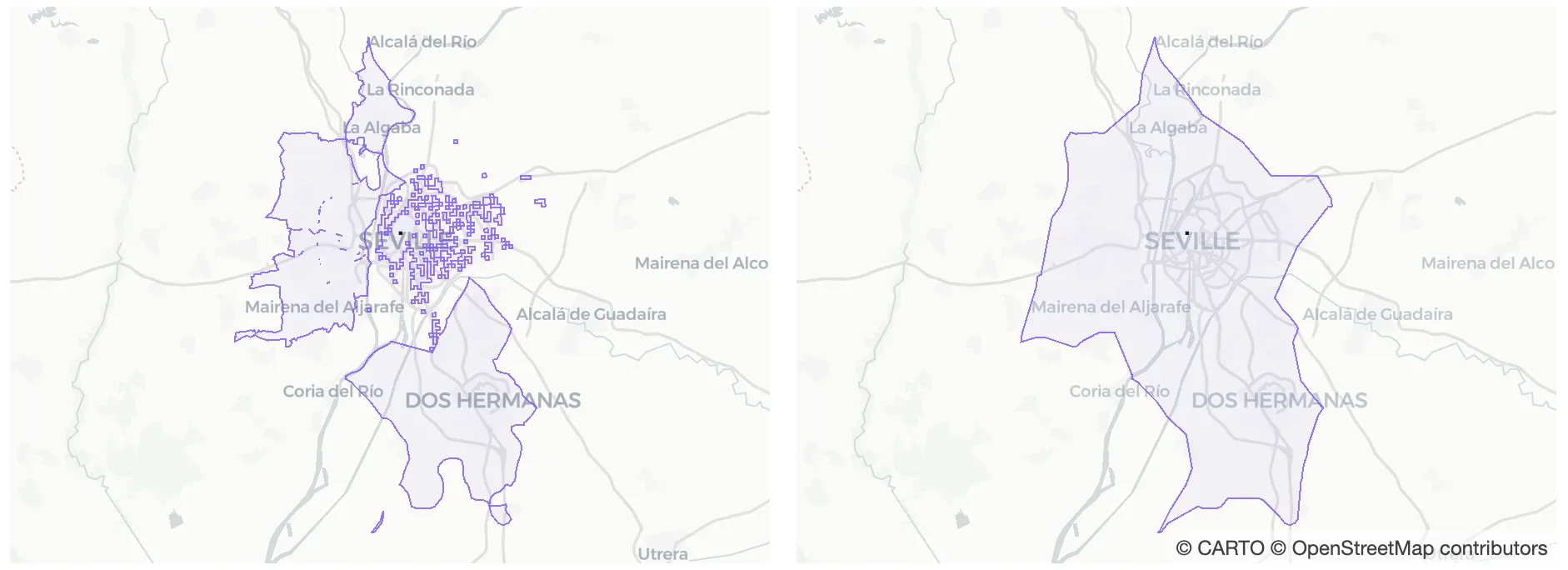
Fig 5. This visualization shows a cell’s raw catchment area and its concave hull.
If we compare the catchment area just obtained with the 15-kilometer buffer and the 20-minute-drive isochrone we can see they look very different from one another. The visualization below shows the three catchment areas with the population cells each of them contains.
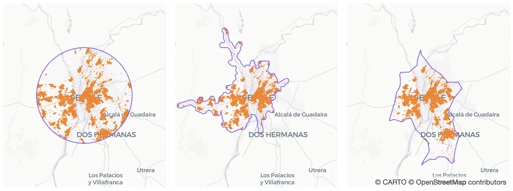
Fig 6. This visualization shows the three catchment areas compared throughout the blogpost and the population cells they contain.
From this comparison we can see how the isochrone expands towards north and west missing a very important urban area in the south of the city which is in fact a very important source of visitors to the destination cell as can be seen in Figure 4. In every iteration of the minimal isochrone process it can be seen that there is a polygon in the south of the city with a very high number of visitors corresponding to this urban area. This area is only partially contained in the buffer catchment area and fully contained by the catchment area we just built using human mobility data.
Tailored Catchment Areas Using Mobility Data
As mentioned above Vodafone Analytics data can be disaggregated by among other variables type of activity at origin (home/work) day of the week and time of the day (morning/afternoon/evening). This gives a lot of flexibility and depending on the business sector or even the use case it may be interesting to use this information to build tailored catchment areas. One example would be to build different catchment areas for weekdays and weekends.
In the figure below we have - for the same target location - the catchment area built using all visits (left) using only visits from Monday through Thursday (center) and using only visits from Friday through Sunday (right). It is very interesting to see how on weekends people tend to travel longer distances than on weekdays.
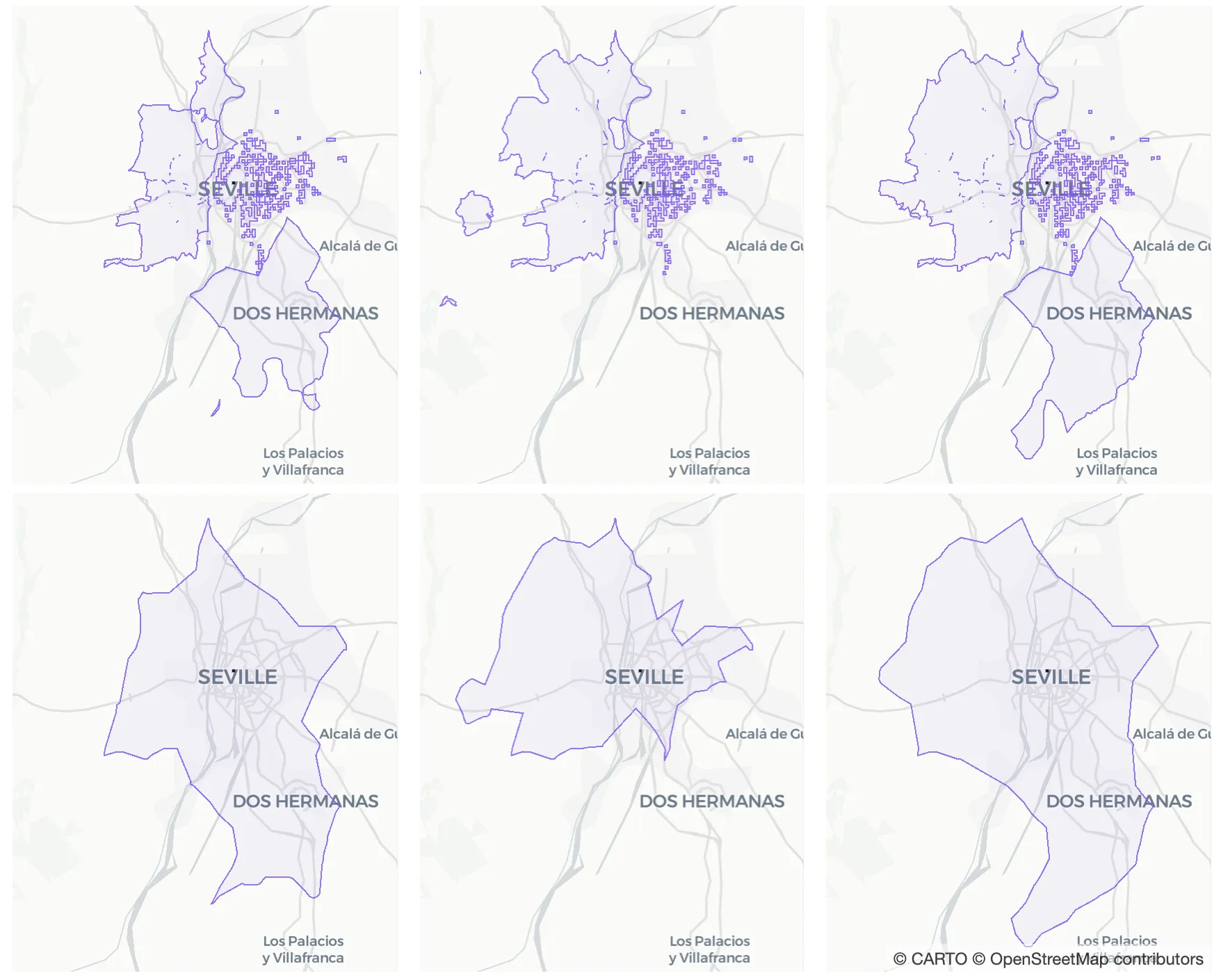
Figure 7. This figure shows target location’s catchment areas considering from left to right all visits visits from Monday through Thursday and visits from Friday through Sunday. Raw catchment areas are in the uppermost row and its corresponding alpha shapes are in the lowermost row right below them.
This level of granularity allows for more powerful business insights. A Real Estate firm using this method is able to provide more detail to potential investors. For a retailer this more accurate catchment can inform decisions around staffing and location management inventory and much more.
For example if we analyze this last level of insight more deeply we can see the catchment area built using weekday visits fits quite well with the 20-minute-drive isochrone while the isochrone based on weekend visits does not (see figure below). This information can be used to identify the right spots to place advertising or have different marketing strategies depending on the day of the week because customers come from different places.
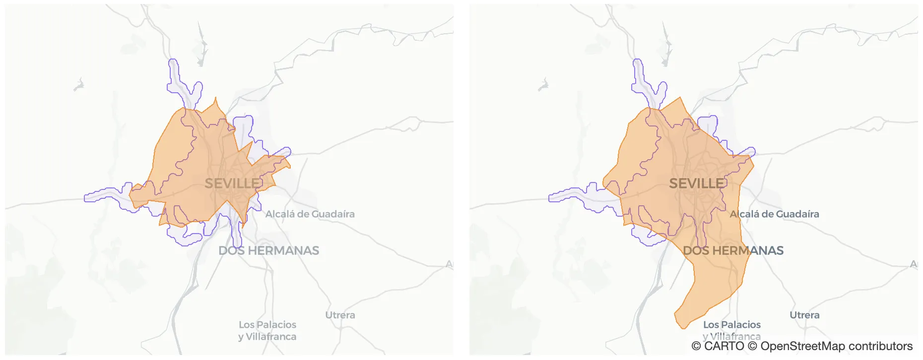
Figure 8. This figure shows catchment areas using weekday visits (left) and weekend visits (right) in orange compared to the 20-minute-drive isochrone (in purple).
Vodafone analytics data can also be disaggregated by sociodemographic variables: age range gender and economic status. This allows for the construction of catchment areas focused on a target customer profile. This can provide even further insight when deciding on store format and retail category.
Deeper insights from Catchment with Human Mobility
Knowing and understanding the characteristics of the areas where a company draws most of its business from is crucial for them to succeed. When starting a new business or expanding an existing one the lack of historical data makes it very challenging to know where customers will come from.
Human mobility data enriched with other location data streams can make a difference when tackling this challenge and help businesses stand out from their competitors.
Special thanks to Mamata Akella CARTO's Head of Cartography for her support in the creation of the maps in this post.
Looking to boost your Spatial Data Science skills? Download the free ebook today!


