What are isolines and how to use them with CARTO


Isolines are an incredibly powerful tool in Location Intelligence, showing the areas that can easily access a given location. You may have also heard these referred to as isochrones trade areas or journey time catchments. No matter their name, the concept is the same - they measure the areas which a site is accessible from based on a set distance or time such as 1 mile or 20 minutes. These calculations are based on traveling along the actual transport network including highways and - where appropriate - cycleways and footpaths.
In this guide, we’ll explain the difference between isolines and fixed-distance buffers, share how you can easily compute isolines, and finally share how you can derive insights from these.
Let’s go!
A fixed-distance buffer is exactly what it sounds like. These compute the catchment of a location based on a fixed distance in every direction from that location. It doesn’t take into account whether travel in all these directions is possible.
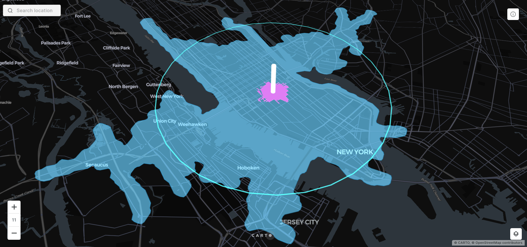
You can see this concept illustrated in the visualization above - the blue circle is a fixed-distance buffer. It doesn’t consider the transport network, and indicates that travel is possible across water.
A fixed-distance buffer has the advantage of being quicker to compute and cheaper to store than the more geometrically complex isolines. However, fixed-distance buffers can be misrepresentative as they assume that all areas within that distance can be easily accessed by individuals. That may not be the case for multiple reasons such as:
- Natural barriers such as coastline, rivers or lakes may obstruct travel.
- Man-made barriers, such as private land, could prevent people from accessing certain areas.
- The network of streets and - if looking at active travel modes - footpaths which comprise an area may not allow for unimpinged travel around a catchment. For example streets may be one way or dead-ends.
With that in mind, are there ever any circumstances where you should use fixed-distance buffers rather than isolines? Absolutely!
One such instance is if you are looking at creating a catchment for a location where you know the transport infrastructure around that location will undergo a major transformation. An example of this would be computing the catchment of a store at a new shopping mall. It is likely that the highway network around that new mall would be completely reconfigured and assessments based on the current network would be completely misrepresentative. In this case a more “indicative" fixed-distance catchment is more appropriate.
Secondly as we mentioned earlier, isolines are more expensive to compute and store than fixed-distance buffers. Additionally, isoline calculations also take advantage of Location Data Services.
Location Data Services - what do I need to know?
The CARTO platform opens up Location Data Services (LDS) to allow you to draw on external APIs to provide extra insight to your analysis.
In the case of computing isolines, CARTO offers this service via our leading partners HERE, TomTom, TravelTime, and Mapbox. These services provide the data driving the transport network that your analysis is run from. You can change to your preferred provider by contacting CARTO directly.
LDS works on a quota system. Each project will have a defined monthly quota, which equates to the number of functions run and the number of features it is run on.
As a CARTO user you can view the status of your LDS quota by running the LDS_QUOTA_INFO() function from the Analytics Toolbox in your data warehouse console. This will tell you information on your project’s monthly total and used quotas, as well as which provider you are using.
Each feature you perform an operation on will consume 1 unit of your quota. So if you ran isochrones from 100 stations, you would consume 100 units. Null values or functions which do not complete due to errors do not consume any units.
Location Data Services also enable a range of other geospatial functions such as geocoding - read more here.
Before diving into creating a catchment, there are a few parameters you’ll need to decide on.
Mode of travel
CARTO’s Analytics Toolbox allows you to select one of two modes of transportation; car or pedestrian.
When selecting "car " your analysis will be limited only to parts of the transport network which allow vehicles. The catchment will also be subject to traffic conditions and restrictions (such as one-way streets) for each street in order to best mimic actual driving conditions.
Conversely when creating a pedestrian catchment more of the transport network will be opened up such as footpaths, cycleways and paths. This analysis also won’t be affected by road speeds or restrictions, but will avoid major highways like interstates and motorways deemed unusable for pedestrians.
As pedestrians and cyclists generally use the same infrastructure you can translate this into analysis for cyclists. Cyclists typically travel 3.75 times faster than a pedestrian, and this figure can be used to scale isolines appropriately e.g. a 30-minute cycle isochrone could be calculated based as an approximate 2-hour pedestrian walk.
You can see the difference between car and pedestrian catchments in the example below originating at the south east corner of Central Park, NYC (the white disk). The green 5-minute walking catchment travels about the same distance in all directions, including through Central Park. Contrasting this is the purple 3-minute walking isochrone which can neither traverse the park nor drive against one-way restrictions, such as along the southbound Fifth Avenue.

Isochrones vs isolines
When creating catchments, there are two main types to choose from; isochrones (catchments based on journey times e.g. how far can I travel in 10 minutes?) or isolines (based on journey distances e.g. how far along the transport network can I travel in 1km?).
When analyzing active travel modes (i.e. walking and cycling), it doesn’t hugely matter which you choose as travelers will typically move at a fairly constant speed. However, if you are looking at a vehicular mode this will matter, as isochrones will be affected by road speeds and traffic conditions whereas isolines will not.
Creating isolines: a guide
Now we are ready to isochrone! These functions are currently available when connected to Google BigQuery, Snowflake and Redshift.
There are three options when running this type of analysis:;
- Use CARTO Workflows, our no-code tool for running multi-step spatial processes. We’ll be focusing on this approach in this blog.
- Use the point-and-click tool in CARTO Builder - learn more in this guide.
- Run the analysis from a SQL console, either in CARTO Builder or your own data warehouse. You can find the code for running isolines with SQL in the LDS module of each Analytics Toolbox.
The results will be exactly the same - it’s cmpletely down to user preference.
If you aren’t already a CARTO user, make sure you sign up for our free two-week trial here!
No-code isolines
No-code isolines
To get started, you’ll need a point layer to act as your catchment origin loaded into CARTO Workflows. If you don’t have a point layer, you can create a central point for your polygon/line using the ST Centroid component. Sorted!
Once we have our point layer, we can compute our catchments.
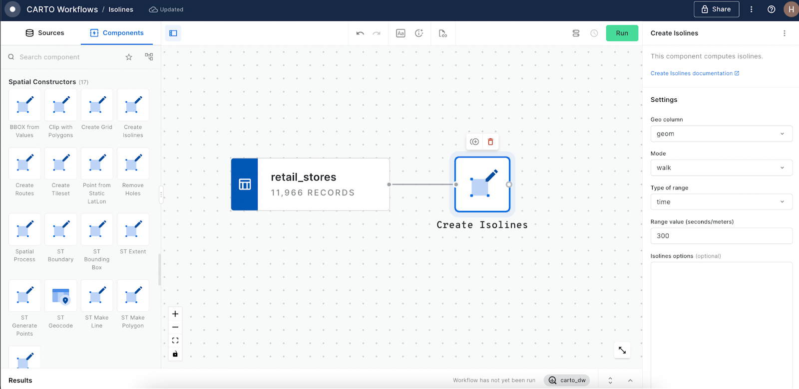
Drag a Create Isolines components onto the canvas, connecting it to your point layer (like in the screenshot below). Fill in the parameters:
- Geo column: this should auto-detect as your point geometry
- Mode: walk/car.
- Type of range: time/distance.
- Range value: seconds/meters.
- Isolines options: set additional options such as arrival and departure time, LDS provider, output detail and more. You can find the additional options available in the LDS module of your cloud’s respective Analytics Toolbox.
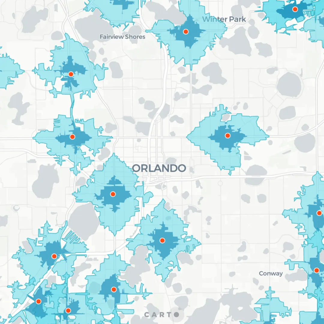
This will create a new table of isoline geometries based on your parameters - such as the example below which shows 15 and 30 minute walk-time catchments from McDonald’s locations in Orlando, Florida.
❗If required, remember to add a Save as Table component to commit your output to a permanent file, as your workflow output will be saved as a temporary file for 30 days.
Deriving insights from isolines
There may be times when producing a trade area is the end goal of your analysis. However, in general, this is just a crucial step to unlock further insights from your analysis.
Below are three examples of the types of insights you can gain from creating isolines.
Insight 1: Isoline characteristics
Being able to understand the number and characteristics of people living or working within a trade area is invaluable. For instance, a retail analyst would be able to assess the size of the potential market of each store based on who could actually travel to their store. They could take this further and work out how many people are likely to walk, cycle or drive to their store and use this to plan parking facilities or focus marketing campaign investments.
A great way to understand this is using CARTO’s Enrichment Tools. These tools allow users to quickly and easily calculate characteristics of an area based on attributes from another dataset - either one of their own or from our Spatial Data Catalog.
Take the example below, where 15 and 30 minute walking isolines are created for McDonald’s in Orlando. Subsequently, these isolines are enriched with the total population from the Census Block Sociodemographics table, available as a free subscription to our users from our Spatial Data Catalog.
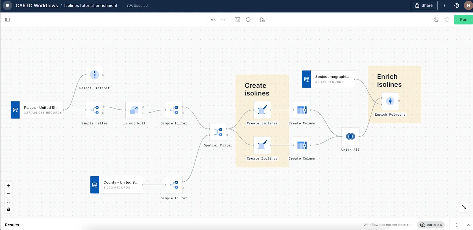
Extending our McDonald’s in Orlando example below, we’ve enriched our 30-minute walking isolines from the previous example with the total population (freely available via the American Community Survey here) as well as a “fast casual affinity" index. This index is available through our data partner Spatial.ai’s Geosocial Segments dataset. It scores people against 72 indexes based on their experiences personalities, feelings shared over social media platforms. Learn more about power of geosegmentation here.
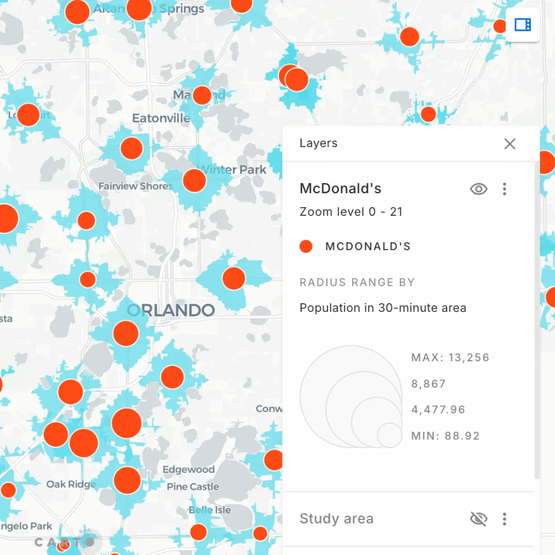
We can use this - along with formula widgets in CARTO Builder - to visualize the differences in demographic characteristics between restaurant catchments.
Insight 2: Reverse trade area demographics
In many cases, it’s not actually the people who have access to a service that you will be most interested in; it’s the people who don’t. Being able to work out where people don’t have easy access to a service is fundamental to strategizing future expansion. In these cases, it’s the areas outside each catchment that is of most interest.
For instance, in the map below the light blue area highlights all of the places in our study area (consisting of the Orange, Osceola and Seminole counties, Florida) which are beyond a 30-minute walk from a McDonald’s. This area can be created using the St Difference component in CARTO Workflows, using isolines and an area of interest as inputs. Using our enrichment tools again, we can calculate that 1,783,500 residents live in this area - approximately 84% of the population!
This figure helps strategists decide whether this study area is a strong candidate for adding additional locations as it has such a large untapped market. The next step would be then to further explore where within the study area would be the optimal location for new stores o services - read more about using CARTO for Site Selection here.

Insight 3: Reverse trade area demographics
Our final insight example is using isolines to assess nearby supporting - or competitive - facilities. Planners behind a new housing development may be required to understand how many relevant services - such as schools, bus stops and health clinics - are accessible within a travel time threshold from their development. Logistics companies may wish to base fleet management decisions or distribution center location on actual proximity to elements of their supply chain.
Building on our example use case, the map below shows the number of other quick service restaurants (QSRs) in the 30-minute walking catchment area of each restaurant to help assess the local competition.
Using a Spatial Join (more details about this here) we can assess competitor brands in each 30-minute walk catchment, and also establish which location has the most competitors. This information is invaluable for driving strategies such as marketing and recruitment.
---
We hope you enjoyed learning about the possibilities of using isolines in your analysis!
If you’re interested in doing more analysis like this, why not explore our human mobility data? A key part of understanding travel patterns is exploring not just patterns of where people could travel, but where they are actually choosing to travel. Request a demo with one of our geo experts to learn more!