Fintech Spatial Data Science Masterclass with J.P.Morgan


Recently we held a DeepFin Investor Tutorial on Spatial Data Science with J.P.Morgan conducted over video conference from London and Madrid. As Spatial data continues to grow in demand across all industries not least in financial services this served as an opportunity to explore specific capabilities and practical applications.
Originally published by J.P.Morgan this summary of the workshop covers three main areas:
- Spatial Data Science
The perception is that Spatial data science simply looks at geo-location data (latitude/longitude co-ordinates) however in practice it includes much more. Specifically spatial data science treats location distance and spatial interaction as core aspects of the data. Spatial data science can be thought of as a subset of traditional data science which focuses on the importance of "where": a special characteristic of spatial data. - Spatial analysis and data science workflows
Using the CARTO spatial analysis framework we are able to 1) Explore: clean geocode and visualise data 2) Enrich: discover and add a wide-range of datasets standardised for spatial aggregations 3) Analyse: get insights to help decisions-makers and 4) Share: output analysis in easy-to-use visualisations. Simply put using spatial data science workflows we can develop spatial models to leverage the special characteristics of georeferenced big data. - Hand-on spatial analysis using Python
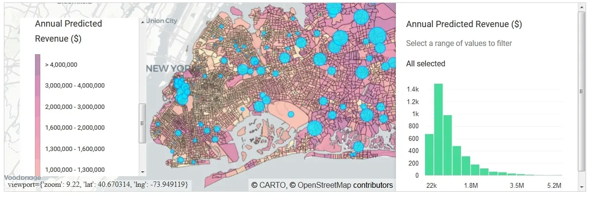
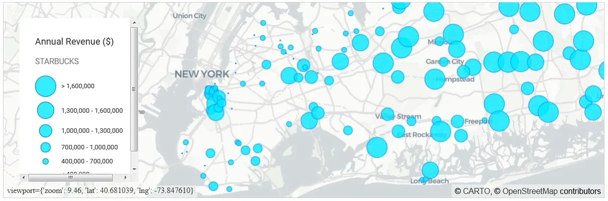
During the practical section of the workshop we went through step-by-step demos using Jupyter notebooks from data exploration to external data discovery and augmentation to model formulation and results. We took at a look at two problems: Site Selection: where should a large coffee chain open its new coffee shops in Long Island? The cover chart shows the annual revenue predictions in Long Island suggesting areas where there is largest prospective revenue potential. Logistics spatial optimisation: where should a parcel delivery company locate their distribution and fulfilment centres? Running an optimisation we propose a new supply chain network with optimal areas for distribution centres measured against distance travelled and average utilisation.
Figure 1: Annual Revenue ($) Predictions in Long Island
Spatial Data Science
Spatial data science treats location distance and spatial interaction as core aspects of the data
Luc Anselin
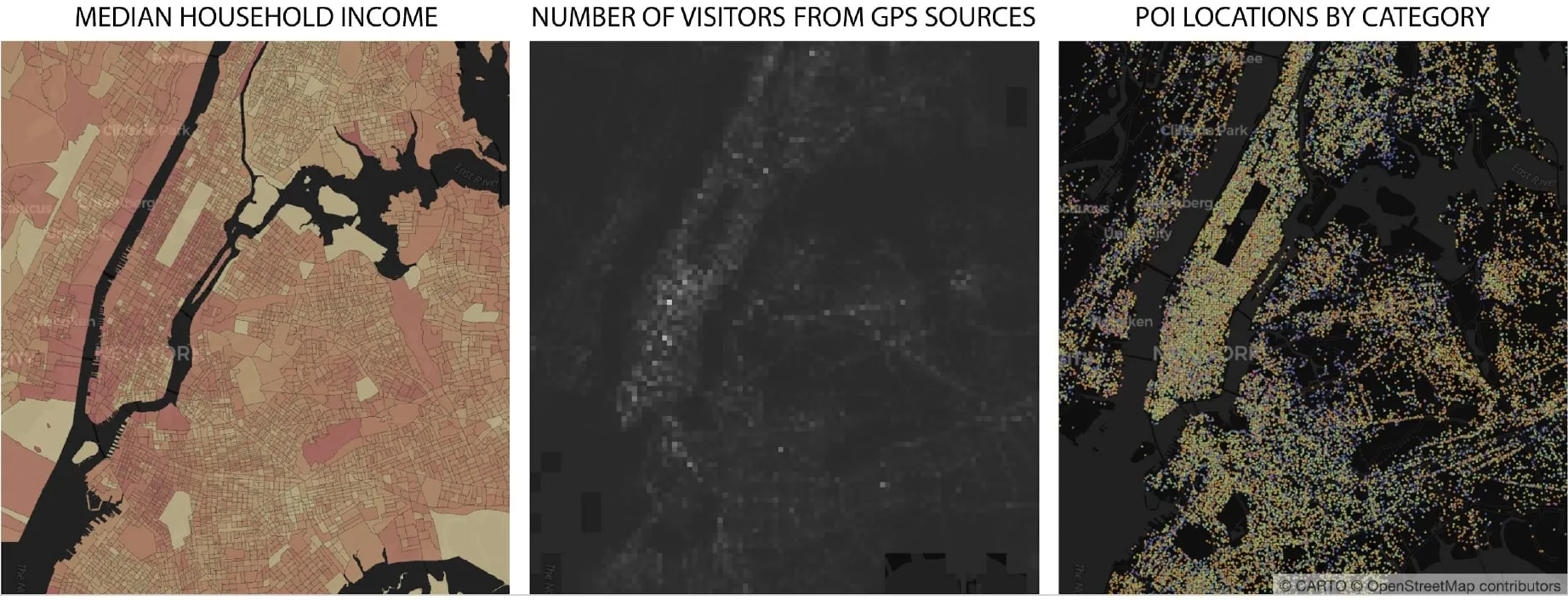
Traditional data science applied to spatial data essentially ascribes no additional value to e.g. longitude / latitude of the data though true spatial data science as above employs specialised methods to work with such data i.e. spatial statistic to statistics spatial databases to databases and geocomputation to computation. Spatial data science can be thought of as a subset of traditional data science which focuses on the importance of "where" a special characteristic of spatial data. Spatial data comes in all forms and shapes e.g. median household income number of visitors from GPS sources POI locations by category - see Figure 2.
Figure 2: Types of Spatial Data
Why is Spatial special? Spatial dependence
One of the useful aspects of spatial data is that data in nearby locations tends to be similar encompassed into the First law of Geography by Waldo Tobler. Essentially spatial data is spatially dependent and independence among observations – a common assumption for many statistical methods – is not present. There are a number of measures of spatial dependence varying on whether you are working with continual spatial processes discrete spatial processes or point-pattern processes.

Spatial Modelling: Leveraging Location in Prediction
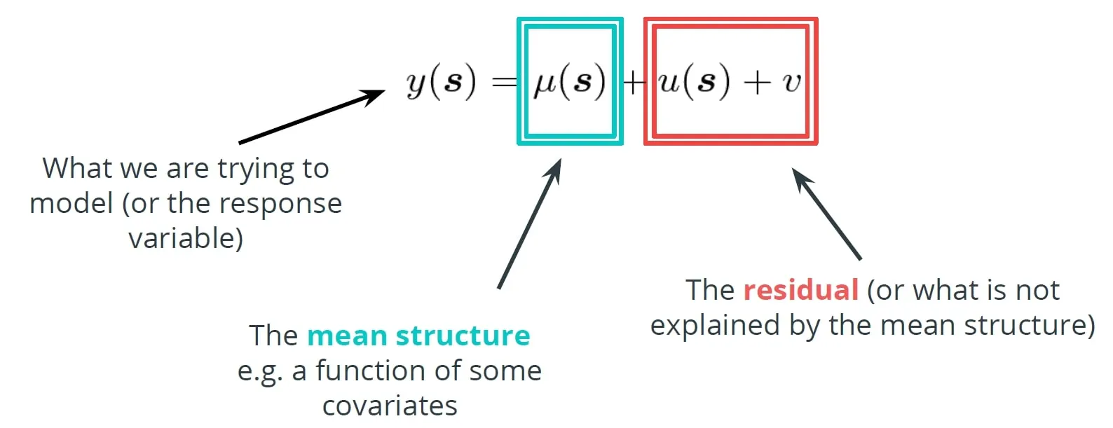
Spatial modelling is similar to classical machine learning in analysing spatial data to make inferences about the models parameters predict unsampled locations and for down/up-scaling applications. Consider a general model of a variable of interest where $$\mu%0$$ is the mean structure and $$ε$$ is an IID process. When dealing with spatial data $$y=y(s)$$ we might add to our general model an extra term $$u(s)$$ representing a spatial random effect acting as a spatial smooth as in Figure 3.
Figure 3: Spatial Modelling
The extra term $$u(s)$$ ensures observations that are close in space will also be "close in" and adds the spatial dependence property
Among common methods when building spatial models include Continuous Spatial Error Models (Gaussian Processes) Discrete Spatial Error Models (Gaussian Markov Random Fields) Spatially Varying Coefficient Models Spatio-temporal models and Spatial confounding.
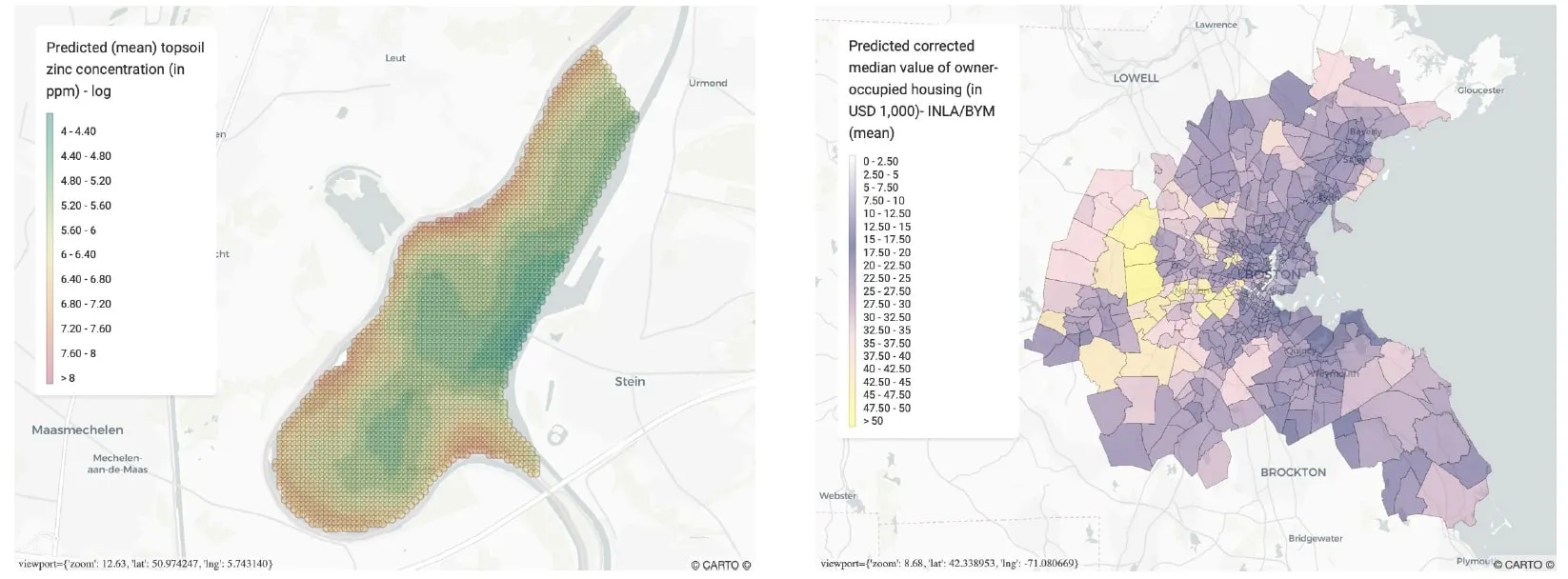
Figure 4: Spatial modelling
a) Continuous spatial error models
The left-hand panel displays a continuous spatial error model of predictions (mean) for the concentration of zinc near the Meuse river in the Netherlands obtained using kriging (Gaussian process regression)
b) Discrete spatial error models
Right-hand panel displays predictions for the owner occupied housing value in Boston obtained using INLA and a Besag York Mollié (BYM) model for spatial random effects
Spatial Clustering and Regionalisation
Akin to clustering in traditional data science spatial clustering adds spatial constraints to ensure geographies are maintained across groups. Such clustering methods which build clusters built from sub-geographies are known as regionalisation.
- Clustering: uses data attributes to create groups that via those attributes are different whilst staying alike with that category. Longitude and latitude can be included as one of these attributes e.g. K-means.
- Spatial clustering: groups together points that are close to each other based on a distance measurement e.g. DBSCAN Generalised DBSCAN.
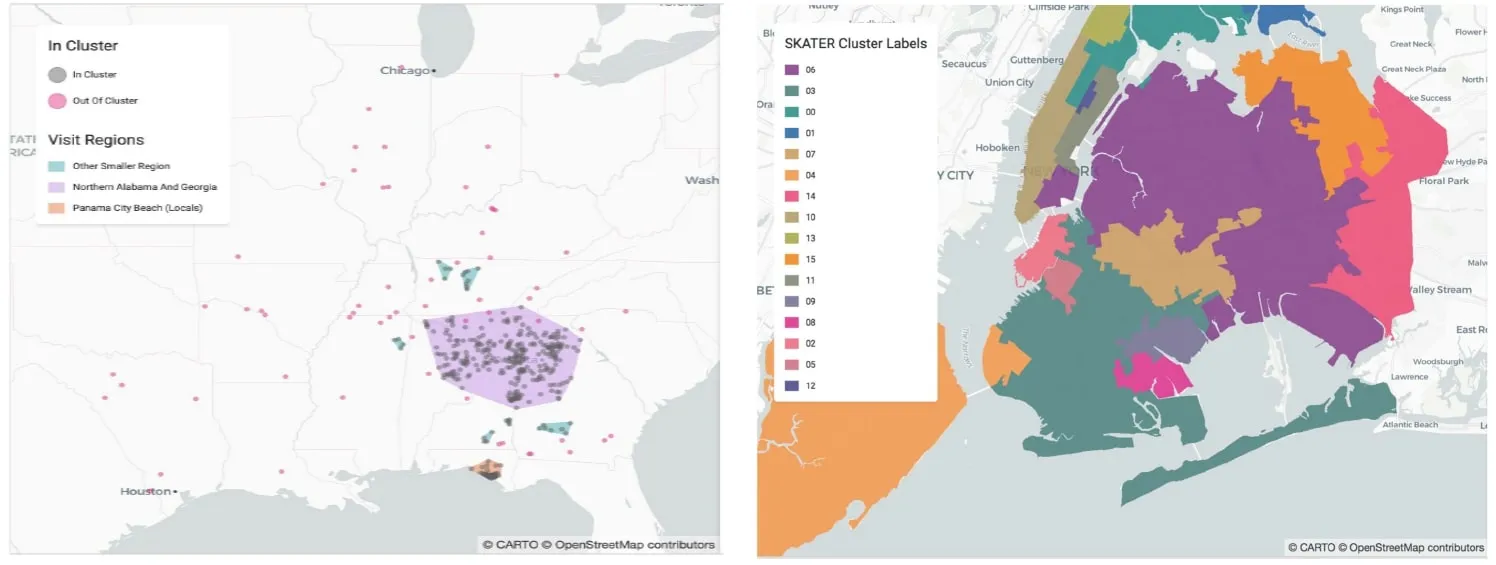
Figure 5: Clustering techniques
a) Clustering
Clustering using DBSCAN: identifies clusters by grouping together items within r distance such that a cluster has m points
b) Regionalisation
Regionalisation enforces contiguity constraints which allows smaller geographies to form larger continuous regions
Practical Spatial Data Science in Python
Using the CARTO tech stack in the hands-on section of the workshop the data scientists from CARTO went through step-by-step demos using Jupyter notebooks from data exploration to external data discovery and augmentation to model formulation and results. The examples addressed two problems:
- Site selection: where should a large coffee chain open new coffee shops in Long Island NY? In this demo we go through a typical site selection use case from modelling the revenues of the existing stores as a function of socioeconomic covariates to predicting the potential revenues in new locations.
- Logistics spatial optimisation: where should a parcel delivery company locate their distribution and fulfilment centres? What areas should they service? In this demo we go through a supply chain network optimisation use case from analysing past data to identify spatio-temporal patterns to building an optimisation model to analyse and quantify the impact of changes in the network.
Want to see this in action?
Request a live personalized demo
Site Selection
Site selection refers to the process of deciding where to open a new or relocate an existing store/facility by comparing the merits of potential locations. If some attribute of interest is known (e.g. the revenues of existing stores) statistical and machine learning methods can be used to help with the decision process.
We start by uploading (dummy) data to CARTO. The data contains the addresses of Starbucks stores their annual revenue ($) and some store characteristics (e.g. the number of open hours per week). Next the addresses are geocoded: we extract the corresponding geographical locations which will be used to assign each store census data of the corresponding block group.
Figure 6: Long Island New York Starbucks locations and Annual Revenue ($)In this problem we use dummy data for store annual revenue
Participants then downloaded the demographic and socioeconomic variables (from the CARTO Data Observatory) that will be used to build a model for the store's revenues. We use data from the American Community Survey (ACS) which is an ongoing survey by the U.S. Census Bureau. The ACS is available at the most granular resolution at the census block group level with the most recent geography boundaries available for 2015. The data that we will use are from the survey run from 2013 to 2017. Further as we are only interested in Long Island for the demo we upload the geographical boundaries of this area from a geojson file.
When comparing data for irregular units like census block groups extra care is needed for extensive variables i.e. one whose value for a block can be viewed as a sum of sub-block values as in the case of population. For extensive variables in fact we need first to normalise them e.g. by dividing by the total area or the total population depending on the application. Checking correlations among the variables there are some noticeably large correlations. To account for missing values and reduce the model dimensionality we transform the data using principle component analysis (PCA).
To understand the relationship between the transformed variables (the PC scores) and the original variable we plot the 10 variables most highly correlated with each PC (see below).
Figure 7: Principle Components correlation scores with the 10 most correlated variablesFor example we see that the first PC which is that dimension that explains the most of the variance is positively correlated with the density of owner occupied housing units but negatively correlated with the density of renter occupied housing units.
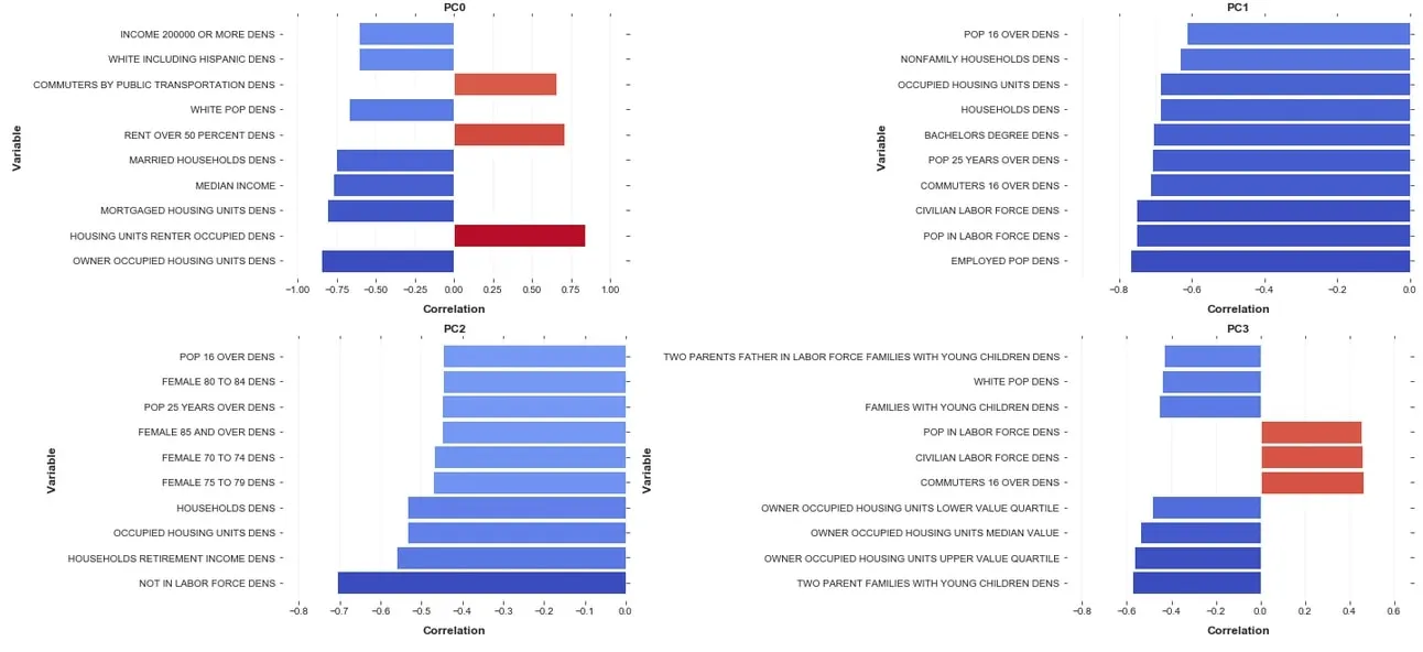
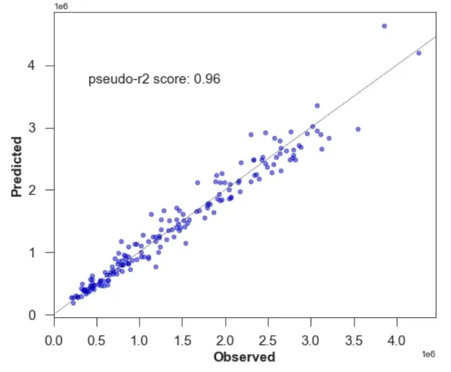
Having prepared the model covariates then we will model the annual revenues by store using a Generalised Linear Model (GLM) with the selected PC scores as covariates. Looking at the model results we notice a significant negative correlation with the first PC (which is lower in richer areas) and a significant positive correlation with the second and third PCs which is negatively correlated with a higher workforce density and a higher density of female seniors. Assessing model accuracy we then plot the observed vs. the predicted values and compute the pseudo-R2 score. As shown in the plot below most data points lie on the 1-1 line and alongside a high pseudo-R2 we can conclude our model is accurate for in-sample predictions.
Figure 8: Testing model accuracy – pseudo R2 for GLM
Finally we can use this model to predict the annual revenue for each block group in Long Island and map the results using CARTOframes.
Figure 9: Annual Revenue ($) Predictions by Long Island block group
Having assessed the performance of the non-spatial GLM model we can check if the model residuals show any residual spatial dependence indicating that better results might be obtained using a model that explicitly takes the property that an observation is more correlated with an observation collected at a neighbouring location than with another observation that is collected from farther away.
Variograms represent a useful tool to check for spatial dependence in the residuals. We fit a variogram models on the residuals by grouping pairs of observations in bins based on their distance and averaging the squared difference from the values of all pairs see Figure 10.
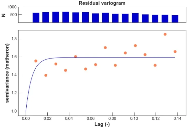
We extend the GLM to account for residual spatial dependence by adding a Gaussian process. Including a spatially-structured random effects model that incorporates such spatial dependency is beneficial when the variables used as covariates in the model may not be sufficient to explain the variability of the observations and the measurements given the predictors are not independent. Fitting the variogram model to the spatial-GLM models’ residuals we can see that we have consistently reduced spatial dependence in the residuals – see the scale of the y-axis in Figure 11.
Figure 10: Spatial dependence in GLM
In the extended model we have removed serial autocorrelation in the residuals.
The next step would be to make predictions using this model though computation time for GPs scale cubically with the data locations this is left for further work.
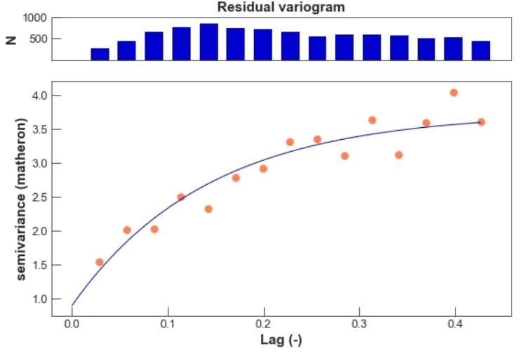
Figure 11: Spatial dependence in spatial-GLM
Logistics Spatial Optimisation: Supply Chain Network Design
Location Intelligence plays a critical role in supply chain network design. From finding better ways to serve stores the optimal location for a new distribution centre or understanding how goods are reaching their final destination every aspect of supply chain design is tied to location data.
Want to see a real world example?
See how SEUR optimized their cold transportation network
In the demo participants walked through all the analytical processes required to build an optimization model to design a supply chain network. In particular we focus on the following steps:
- Assess the current state: identify where there is more demand the characteristics of high order concentration areas and whether distribution centres (DCs) are strategically located.
- Assess and quantify the impact of changes in their current network. Mainly the impact of opening/closing DCs and changes in delivery areas.
- Build an optimisation model to identify where DCs should be located and design their transportation network (supply chain network design).
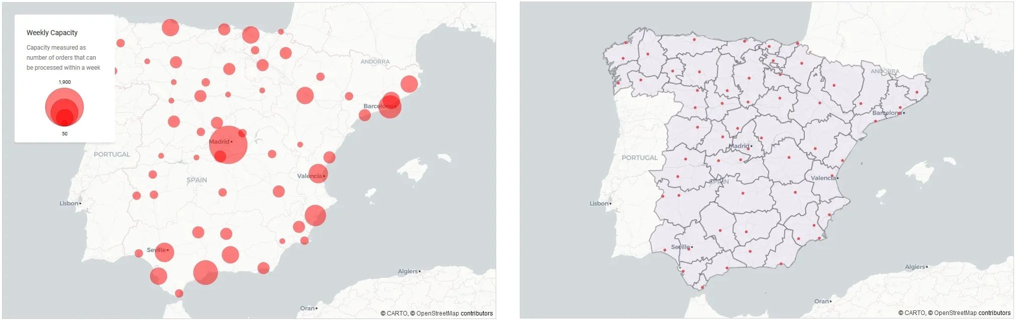
Firstly we load the current distribution network data including their locations capacity and operational areas. The current network operates based on regional administrative regions as we can see Figure 12.
Figure 12: Distribution Centres | Locations and capacity (left panel) and current operational areas (right panel)
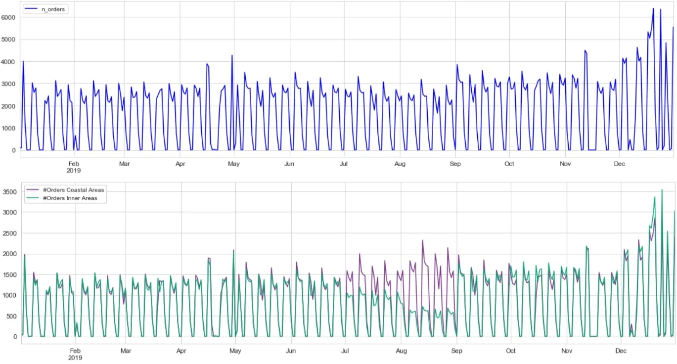
Next we look at the last year’s geolocated historical order data. Looking at the number of orders on its own – a temporal analysis of orders – shows the variability of orders. Adding the spatial component into the analysis to now run spatio-temporal analysis of orders shows the demand series varies not only by time but also by location. In the summer months the number of orders from inner areas recedes as the number of orders from coastal areas increases.
Figure 13: Number of orders – temporal (top panel) and spatio-temporal analysis (lower panel)
The first analysis we will carry out is a clustering analysis to identify areas with a high concentration of orders. The goal of this analysis is to verify whether DCs are strategically located and whether the spatial characteristics of high density areas (land covered administrative areas covered etc.) can be leveraged to improve delivery areas.
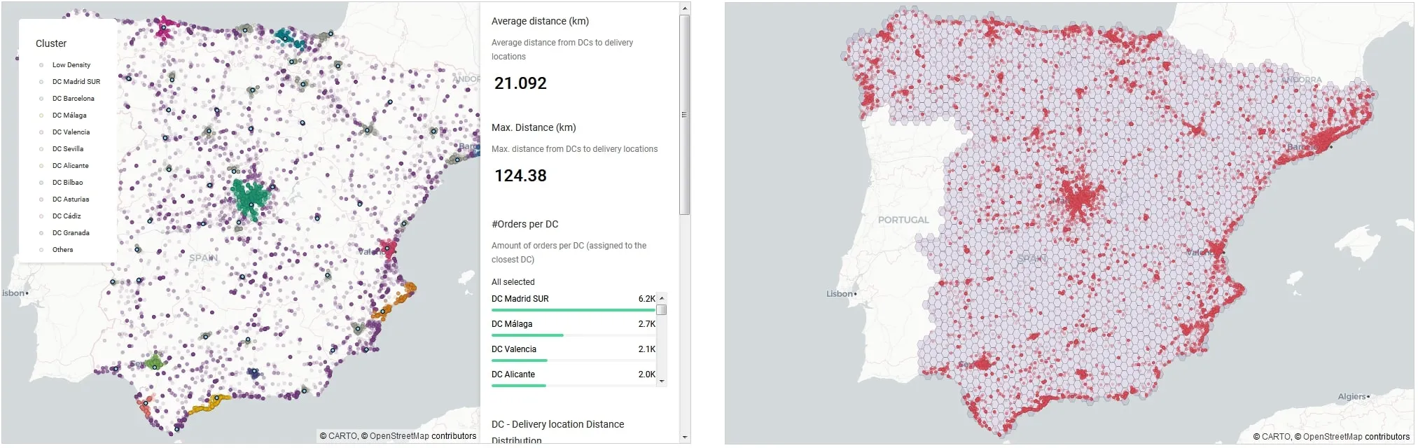
For this analysis we will use DBSCAN a density-based clustering non-parametric algorithm which groups together points that are closely packed together (points with many nearby neighbours) marking as outliers points that lie alone in low-density regions.The map below shows the clusters obtained with a sample of orders. It can easily be seen how different patterns emerge such as:
- Long areas along the coast (Málaga Alicante)
- Compact areas around large cities (Madrid Valencia)
- Large areas of low concentration of orders.
The panel on the right displays spatial intersections and spatial aggregations.
Figure 14: Supply-demand matching - analysis of the current SC network
For strategic and tactical planning the focus is not on the exact location of orders but rather an estimation of them aggregated both spatially and temporally. Selecting the right spatial aggregation is critical.
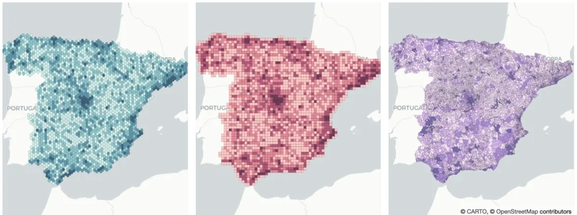
There are different alternatives for spatial aggregation. H3 and Quadkey grid are two examples of standard hierarchical grids. However oftentimes business requirements impose the use of other spatial aggregations more "natural" to people.
Some examples are zip codes municipalities and administrative regions.
Figure 15: Spatial aggregation methods H3 (left) Quadkey (middle) and natural (right)We aggregate orders delivered using H3 Quadkey grids and municipalities.
We move onto building an optimisation model to calculate the optimal delivery areas of each DC so that they could be compared to existing ones. The linear optimisation model has the following costs in the objective function:
- Average distance travelled
- Deviation from a perfect balance of workload in the DCs during the peak season i.e. we penalised having some DCs at 200% of their capacity while having some others at 50% for example.
- Deviation from a perfect balance of population covered by distribution centre capacity.
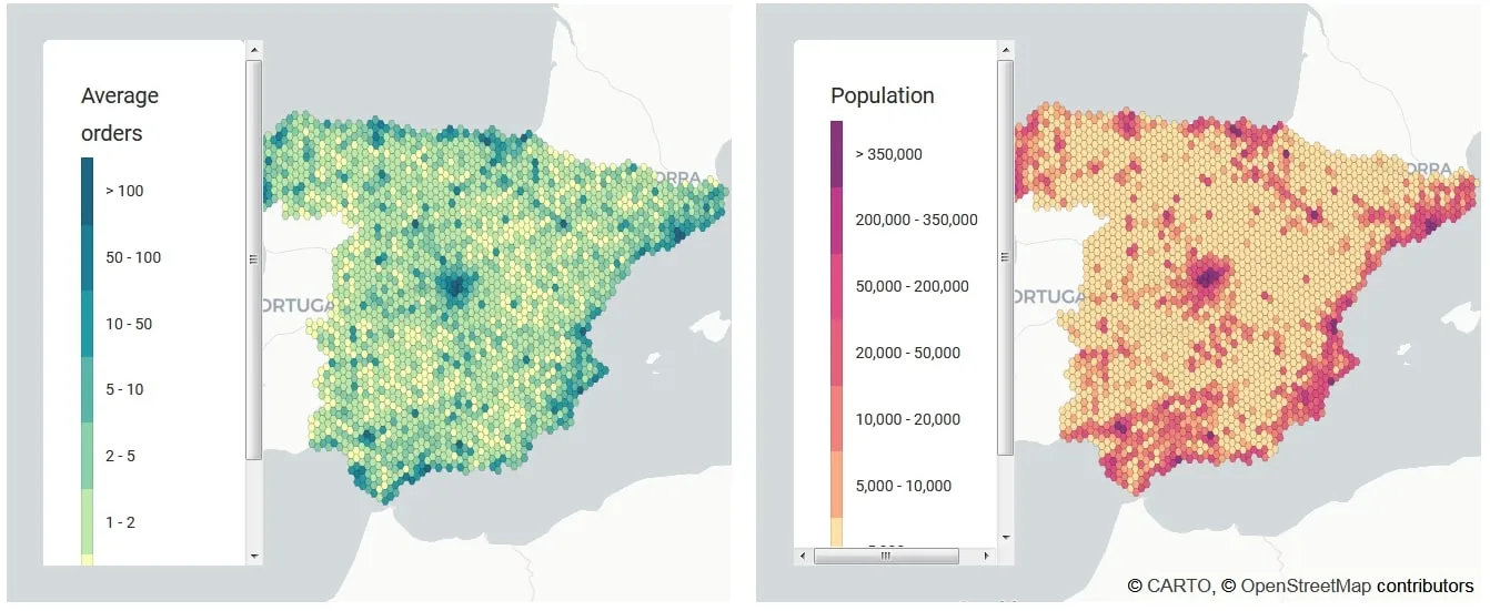
To allow us to meet the third constraint we enrich our dataframe with WorldPop data to ensure that the population covered by each DC is evenly distributed with regards to the DC capacities. The enriched dataframe is visualised in Figure 16.
Figure 16: Average orders and population dataThe two panels here display average orders across Spain alongside population density
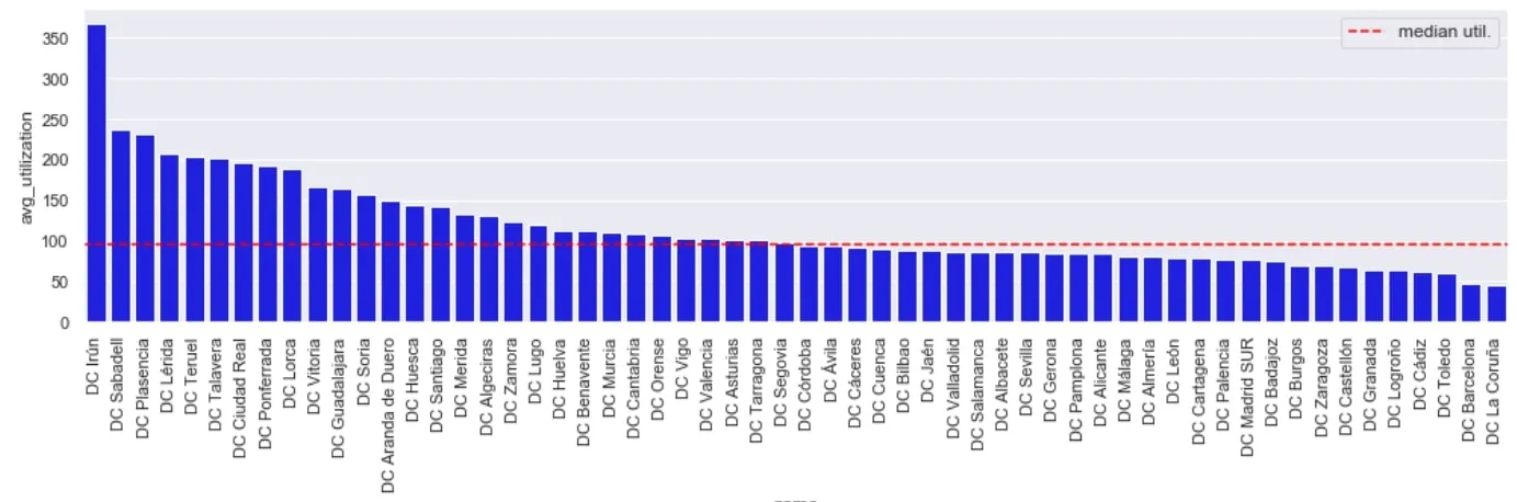
Given our enriched dataset we can now check the current utilisation in the supply-chain network. We can see there are a number of DCs where the average utilisation is >150% of capacity. The aim of the optimisation would be to calculate optimal delivery areas of each DC.
Figure 17: Current utilisation across DC supply-chainBy in large most DCs operate below capacity but there is a notable number where average utilisation is >150% of capacity
After running the optimization algorithm the optimal areas for DCs can be seen in the right panel in Figure 18 – compared to the current areas based on administrative regions (left panel). Interestingly whilst the average DC utilisation comes down from 124% to 116% the distance travelled increases from 21km to 27km. This would suggest some DCs (e.g. Sabadell) may benefit from additional DC space.
Figure 18: Current operational areas (left) and optimal operating areas (right)The left panel display the current operational areas of DCs whilst the right panel displays proposed optimal operating areas
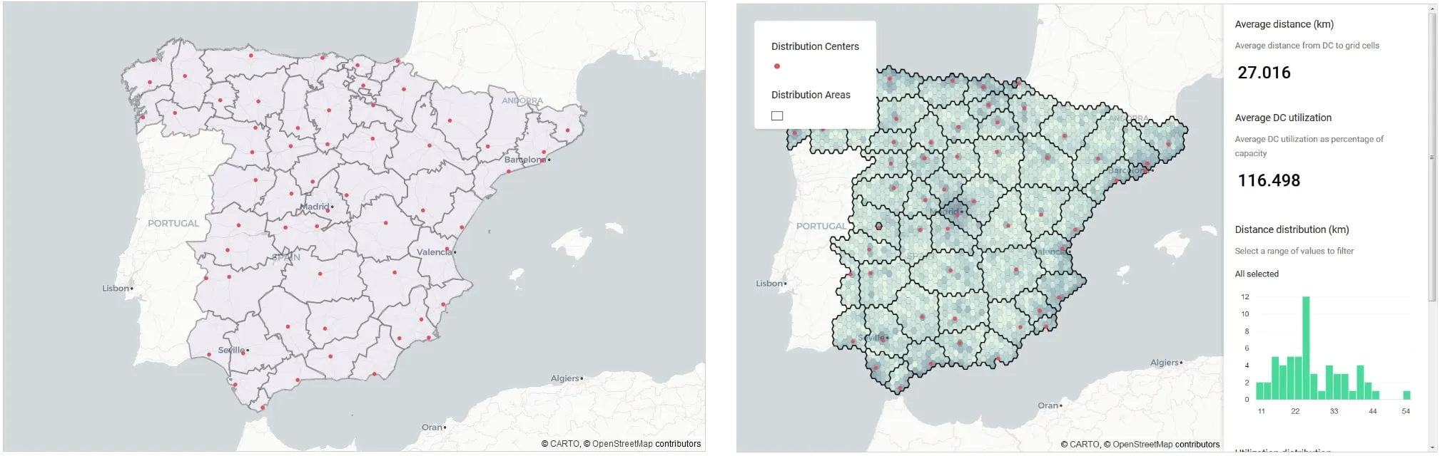
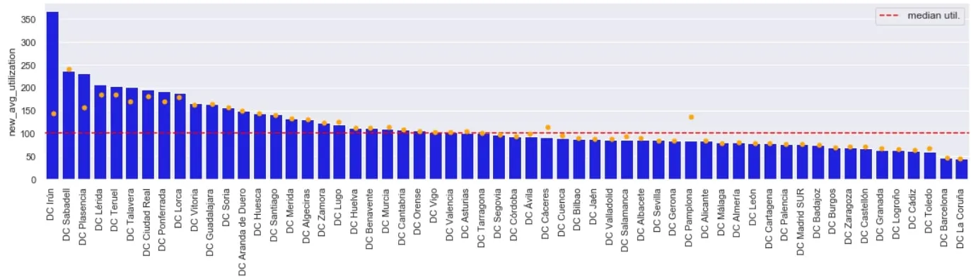
Figure 19: Optimal new average utilisation (orange dots) across DC supply-chainBy in large there is a significant reduction in average utilisation across the SC as depicted by the orange dots for each DC
Takeaways
- Spatial data science treats location distance and spatial interaction as core aspects of the data.
- Spatial data science can be thought of as a subset of traditional data science which focuses on the importance of "where": a special characteristic of spatial data.
- Spatial data comes in all forms and shapes e.g. median household income number of visitors from GPS sources POI locations by category.
- Spatial modelling leverages location in prediction and is similar to classical machine learning in analysing spatial data to make inferences about the models parameters predict unsampled locations and for down/up-scaling applications.
- E.g. spatial clustering groups together points that are close to each other based on a distance measurement
- Regionalisation is an extension of spatial clustering which enforces contiguity constraints allowing smaller geographies to form larger continuous regions
- CARTO’s framework provides the ability to explore enrich analyse and share data.
- When looking at site selection we can use spatial modelling of revenues of existing stores as a function of socioeconomic covariates to predict potential revenues of new locations.
- Running an optimisation we propose a new supply chain network with optimal areas for distribution centres measured against distance travelled and average utilisation.
Want to get started?