Fuel Shortage UK Maps & What Location Data Can Tell Us

In September 2021 many petrol stations across the UK ran out of fuel. Panic buying was attributed to media reports of a leaked government briefing outlining the shortage of heavy goods vehicle (HGV) drivers. Some analysts and politicians linked the driver shortage to Brexit  whilst others blamed the COVID-19 pandemic  or a combination of both of these factors.

But were the long queues at petrol stations across the UK caused by legitimate shortages or as a result of panic buying fueled by over zealous press reports? In a recent webinar with Unacast we explored the real story in order to try and answer this question along with several others such as:

• How has consumer behavior changed in reaction to supposed petrol shortages?
• Just how much longer are the queues at the pump?
• Which brand suffered the longest wait time for fuel?
• Is it quicker to fill up in the city  the country  or the suburbs?
• Which areas of the UK are most prone to panic buy?

Want to see this in action?

Watch the webinar on demand

First we selected a sample of petrol stations located in and around the London area which included a number of different brands such as Shell, Texaco, and BP. The sampled petrol stations can be seen in the map below.

Map(Layer(stations  
          geom_col='geometry' 
          style=color_category_style('location_name_g'  size=6  stroke_width=0  opacity=0.95  
                                     cat=['Shell'  'Texaco'  'BP'  'JET'  'ESSO']  
                                     palette=['#F2B701'  '#DF0909'  '#73AF48'  '#1D6996'  '#7F3C8D']) 
          legends=color_category_legend('Petrol Brand') 
          popup_hover=[popup_element('location_name'  title='Location Name') 
                       popup_element('address'  title='Address') 
                       popup_element('city'  title='City')]))

With these locations Unacast was able to extract activity data during a period of two months between August 1 2021 and October 1 2021. The resulting map shows the activity data around these locations.

Map([Layer(activity  
           geom_col='geometry'  
           style=basic_style(color='#E73F74'  opacity=0.33  stroke_width=0) 
           legends=basic_legend('Activity data'  'SDK signal locations'  
                                footer="""<p>Zoom in to visualize a station's activity</p> 
                                          <p><b>Source</b>: Unacast</p>""")) 
     Layer(stations  
           geom_col='geometry'  
           style=basic_style(stroke_color='#F2B701'  stroke_width=1  opacity=0  size=15) 
           popup_hover=popup_element('address'  'Station') 
           legends=basic_legend('Petrol Stations'  'Sample petrol station locations'))] 
    basemap=basemaps.darkmatter)

We wanted to understand if the dwell time  i.e. the amount of time people were spending queuing for fuel, had increased during this period of time and so first we plotted the average dwell time (aggregated by week to avoid any noisy data). The graph below shows that starting on the week beginning September 29 we can see a significant increase in dwell time which keeps growing until October 19.

plt.figure(figsize=(12 4))
gact = activity.set_index('local_event_date').resample('W').mean()
gact['duration_seconds'].plot(color='red'  linewidth=1)
plt.ylabel('Average duration')
plt.xlabel('')

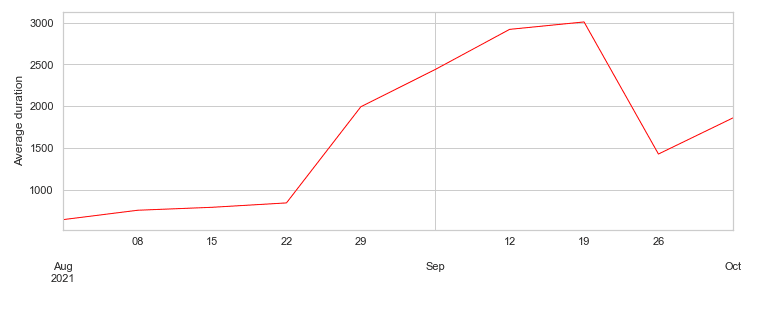
The decrease and increase towards the end of the selected time period is driven by some outliers and so the next step was to clean the data in order to focus on the petrol stations that could provide higher quality and more stable data. At this stage our hypothesis that dwell times are increasing due to shortages reported in the press appears to hold true but we wanted to disaggregate this information at the location level to see if this is happening on a wider scale or if there are any observable patterns.

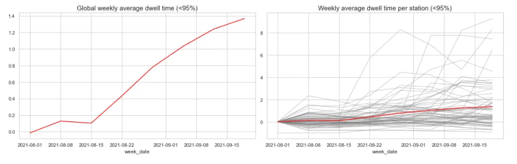
To do this we selected the first week of August as our baseline and then calculated the increase or decrease in dwell time accordingly. In the graphs below we removed the top 5% that exhibited the largest increases since they dominated the sample and we can see in the graph on the left that dwell time started to increase on a constant basis from the week of September 22 within London. The red line on the graph to the right represents the average dwell time and shows us that this is not happening in a regular manner in every station  i.e. there are some specific petrol stations that have been affected more than others.

# double plot because we lose some information

fig  axs = plt.subplots(1  2  figsize=(20  5))

sts.loc[(sts[sts.columns[1:]] < sact['duration_rel'].quantile(0.95)).sum(1) == 9  sts.columns[1:-1]].transpose().mean(1).plot(figsize=(16 5)  color='red'  ax=axs[0])
axs[0].set_title('Global weekly average dwell time (<95%)'  fontsize=15)

sts.loc[(sts[sts.columns[1:]] < sact['duration_rel'].quantile(0.95)).sum(1) == 9  sts.columns[1:-1]]\
    .transpose().plot(figsize=(16 5)  color='grey'  legend=False  linewidth=1  alpha=0.5  ax=axs[1])
sts.loc[(sts[sts.columns[1:]] < sact['duration_rel'].quantile(0.95)).sum(1) == 9  sts.columns[1:-1]]\
    .transpose().mean(1).plot(figsize=(16 5)  color='red'  ax=axs[1])
axs[1].set_title('Weekly average dwell time per station (<95%)'  fontsize=15)
fig.tight_layout()

To try to understand this more and identify any additional patterns we then performed a spatio-temporal analysis in order to plot this behavior on a map and see how it evolves over time. This resulted in the animated map below showing the change in dwell time over the two months.

‍

Map(Layer(fmsts  
          geom_col='geometry'  
          style=size_continuous_style('duration_change_new' 
                                      animate='date' 
                                      size_range=[5 100] 
                                      opacity=0.25 
                                      color='red' 
                                      stroke_color='red' 
                                      stroke_width=0) 
          legends=size_continuous_legend('Change in dwell time' 
                                         description='Percentage of change in dwell time wrt to first week of August' 
                                         footer='Source: Unacast') 
          widgets=animation_widget('date')) 
    basemap=basemaps.darkmatter)

‍

Observing this map we can see some interesting trends  such as a large initial increase at the start of August around the Luton area with increases in other parts of the city taking effect later on during early September. We can also identify some areas that have petrol stations with the highest increases alongside nearby stations where dwell time has remained static which may indicate some degree of territory organization between the brands in order to ensure better supply. The map shows us that the pattern is not uniform across the city and even towards the end of the selected time period we see sudden increases in the dwell time at a number of locations.

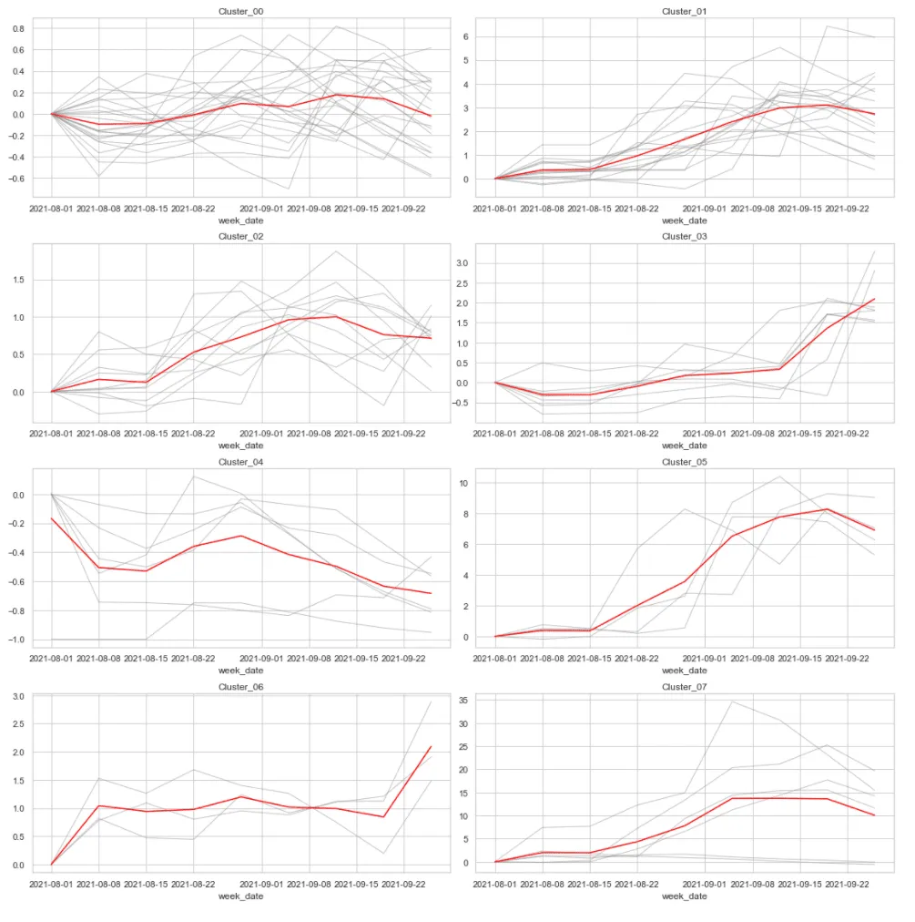
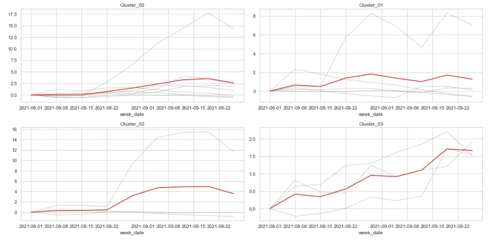
Next we grouped the petrol stations into homogenous groups  i.e. those exhibiting similar behavior  to identify where they were located and gain additional insights. By using time series clustering we identified 8 clusters that exhibited similar behavior. For example cluster 0 includes petrol stations where the change was not important and stayed relatively the same during the time period  whereas clusters 1 and 5 exhibit much more important increases of 3x and 8x respectively.

fig  axs = plt.subplots(4  2  figsize=(16 16))
for i in sts['fcluster'].unique():
    sts.loc[sts['fcluster'] == i  sts.columns[1:-3]].transpose().plot(
        color='grey'  legend=False  linewidth=1  alpha=0.5  ax=axs[i//2  i%2])
    sts.loc[sts['fcluster'] == i  sts.columns[1:-3]].transpose().mean(1).plot(
        color='red'  ax=axs[i//2  i%2])
    axs[i//2  i%2].set_title(f'Cluster_0{i}')

fig.tight_layout()

‍

One question posed earlier was if this activity was dependent on petrol brand and if we plot clusters by brand we can see that the top brands have petrol stations in most clusters  experiencing very different behaviors  meaning there is little or no dependence.

plt.figure(figsize=(14  4))
sns.countplot(x='location_name_g'  hue='cluster_cat'  data=stations_c  hue_order=np.sort(stations_c['cluster_cat'].unique()))
plt.legend(loc=1)

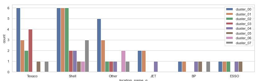
Plotting the clusters on a map shows us that they don’t depend on location  with clusters spread throughout the city. For example in the suburbs south west of London  towards Sandhurst  there are three petrol stations exhibiting a significant change with two others in clusters without such a change. This reflects what we saw in the animated map and there does not appear to be a spatial pattern. For example both clusters 0 (no significant change) and 5 (significant change) have locations within both the city center and suburbs showing no significant pattern. Again selecting one of the brands within the map shows different clusters across location.

Map(Layer(stations_c  
          geom_col='geometry'  
          style=color_category_style('cluster_cat'  
                                     palette=palettes.bold 
                                     cat=list(np.sort(stations_c['cluster_cat'].unique())) 
                                     stroke_width = 0  
                                     size=8 
                                     opacity=0.95) 
          legends=color_category_legend('Petrol Shortage Impact' 
                                        description='Petrol stations in the London Area' 
                                        footer='Source: Unacast') 
          widgets=[category_widget('cluster_cat'  title='Cluster'  description='Select one cluster') 
                   category_widget('location_name_g'  title='Petrol brand'  description='Select one brand')]))

Given there is no significant pattern observable we would need some additional external data in order to explain exactly what is happening. However as a final step we wanted to identify if there was some coordination between petrol stations that were very close to each other. Therefore based on the sample  we took four spatial clusters close to one another and analyze what was happening.

Map([Layer(spatial_clusters_f  
           style=basic_style(opacity=0  stroke_width=2  stroke_color='#000000') 
           widgets=category_widget('cluster'  'Spatial Cluster')) 
     Layer(gpd.sjoin(stations_c_f  spatial_clusters_f) 
           style=color_category_style('cluster_cat'  
                                     palette=palettes.bold 
                                     cat=list(np.sort(stations_c['cluster_cat'].unique())) 
                                     stroke_width = 0  
                                     size=8 
                                     opacity=0.95) 
          legends=color_category_legend('Petrol Shortage Impact' 
                                        description='Petrol stations in the London Area' 
                                        footer='Source: Unacast') 
          widgets=[category_widget('cluster_cat'  title='Dwell Time Clusters'  description='Select one cluster') 
                   category_widget('location_name_g'  title='Petrol Brands'  description='Select one brand')])])

What we observed was that for the first three spatial clusters there was one petrol station which experienced a very important increase in dwell time whilst the others remained roughly the same. This is interesting as it tells us there might be some coordination between stations or certain social behaviors being exhibited (e.g. people are more likely to congregate at a petrol station they see with a big queue since they believe it will have fuel).

fig  axs = plt.subplots(2  2  figsize=(16 8))
for i  row in spatial_clusters_f.iterrows():
    address_f = list(stations_c_f.loc[stations_c_f.intersects(row['geometry'])  'address'].values)
    sts.loc[sts['address'].isin(address_f)  sts.columns[1:-3]].transpose().plot(
        color='grey'  legend=False  linewidth=1  alpha=0.5  ax=axs[i//2  i%2])
    sts.loc[sts['address'].isin(address_f)  sts.columns[1:-3]].transpose().mean(1).plot(
        color='red'  ax=axs[i//2  i%2])
    axs[i//2  i%2].set_title(f'Cluster_0{i}')

fig.tight_layout()

By using data in this way it allows us to link press reports with real world activity and determine the real story. We’ve been able to confirm that dwell times were increasing due to increased demand and therefore shortage of fuel. Was it happening everywhere? No. Did it depend on the petrol brand? It seems not (it could be there was some coordination between brands). The patterns we have found are very heterogeneous which help us to go further and ask more questions and go further. For example we could enrich our data with activity type around the areas of interest relating to commercial or recreational activities.

Want to get started?

Sign up for a free trial accoung

This project has received funding from the European Union's Horizon 2020 research and innovation programme under grant agreement No 960401.