How to Improve Retail Trade Area Accuracy with Mobility Data

In the retail industry a trade area  also known as a catchment area  is the geographic area from where you draw your customers. There are a number of methods for calculating such an area including using buffers or drive times. As retailers look for a more accurate picture of their customers and competitors they are combining these more conventional methods with new types of location data. Human mobility data in particular can give a significant boost to the accuracy of catchment areas compared to the economic and demographic data from conventional drive time trade areas. Using the example of Costco in the Bay Area  this post looks at how this can be achieved by analyzing and visualizing SafeGraph mobility data.

A Mini Background on Catchment Areas

In the field of Watershed Science and Ecology  a catchment area typically refers to ‘land which is bounded by natural features such as hills or mountains from which all runoff water flows to a low point’. It’s easy to picture how gravity will naturally carry water to a low point. This gravity-based model of a catchment area has since been applied to human geography and is a core tool in geospatial analysis. The Huff Gravity Model takes this further by offering a formula for calculating the probability for how many consumers will go to one store (over another) based on distance and size of the store. We commonly use catchment or trade areas to understand the area that a location serves or draws visitors from.

From Buffers to Drive times

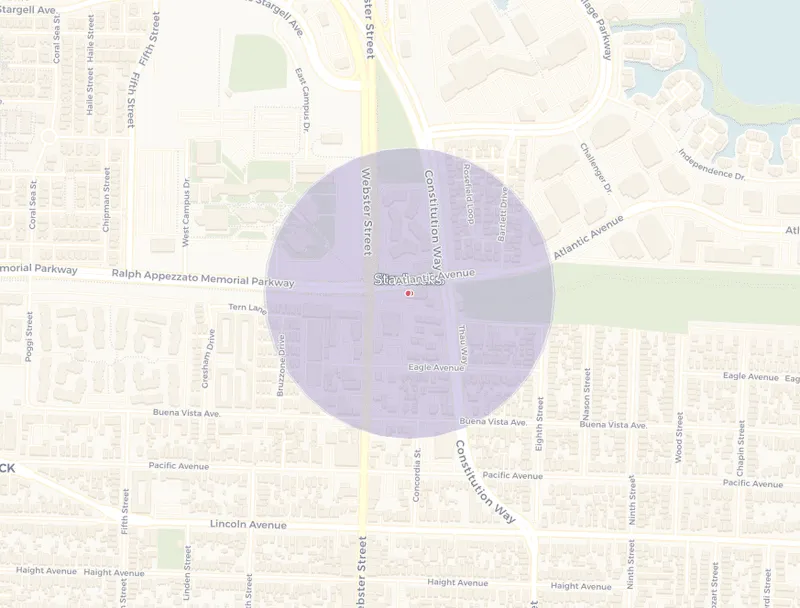
A simple example of a trade area would be one for a post office or a Starbucks. While the odd person might indeed enjoy driving a long way to go to a location in another city  most people will go to the closest one. By drawing a circular 2km buffer around a location  we can get a general picture of the population that location serves.

Isochrones or drive times allow us to generate a trade area based on the average distance covered by different modes of transport (e.g.  walk  bike  or drive). This gives us a more accurate picture that accounts for travel time differences. If one Starbucks is a 30 minute walk away and the other is a 10 minute walk  you’re more likely to go to the closer one.

What Human Mobility Data Offers

Human mobility data gives us an anonymized and an aggregated picture of where people go during the day and where they live (i.e.  where their device remains at night). There are a wide variety of human mobility data providers out there and one of the providers we work with frequently is SafeGraph. SafeGraph’s Patterns data shows us many things  the most important of which is where a store’s visitors came from. For every point-of-interest (POI) in SafeGraph’s system  we can see which census block group the visitors live in and the count of visitors coming from that block group. While other mobility providers often give us raw lat/long ping data  SafeGraph does the aggregating and cleaning work for us.

This data is immediately valuable with the right geospatial tools. Each row contains a store or brand location with information about the visitors. When we plot these visitor block groups on a map  the result is incredible. We suddenly have a much more accurate picture of a store’s trade area compared to a buffer or drive time. Rather than seeing a simplified drive time or buffer shape on a map  we can actually see the areas where people came from. The next step is enriching those block groups with other data (like Census Demographic data) so we can learn something about the people who live in those block groups. This will allow us to understand the differences between the customers at each location.

A Short Trade Area Enrichment Comparison

Enriching a trade area involves joining the trade area geometry to another dataset based on a spatial relationship (in a spatial join) or a shared column (in an attribute join). We commonly enrich trade areas using the US Census American Community Survey Data (ACS) to understand the demographic and economic characteristics of those block groups.

I wanted to see if there was a measurable difference between enriched drive time trade areas and human mobility data trade areas. I calculated the median income of 15 different Costco stores by enriching their drive time trade areas.

Here are the 15 Costcos and their respective 10-minute drive times:

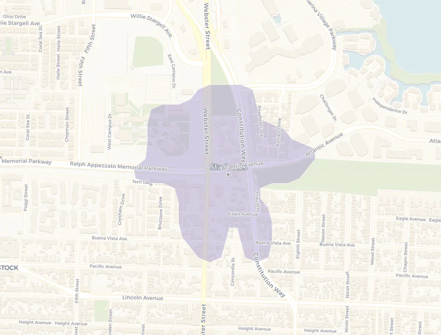
Now here’s a map of all the home visitor block groups (from SafeGraph) for those same Costco stores. I filtered out the block groups with fewer than 5 visitors to give a stronger sense of where the visitors come from. The map allows you to filter by the placekey for each store if you want to see only one.

The next step is enrichment. I used CARTOframes’ enrichment capabilities to enrich the drivetime polygons using the ACS data. To enrich the mobility trade area area  I used a Python function to calculate the weighted average -- the weighted average ensures that a block group which has 100 visitors (for example) has a greater proportional effect on the average compared to a block group that has 5 visitors.

The complete analysis can be viewed in this Python notebook.

Results: Median Age Differences between Drive time vs. Human Mobility Data Trade Areas

For Costco’s in the Bay Area  the median income looks very different depending on whether you use drive time or human mobility data trade areas.

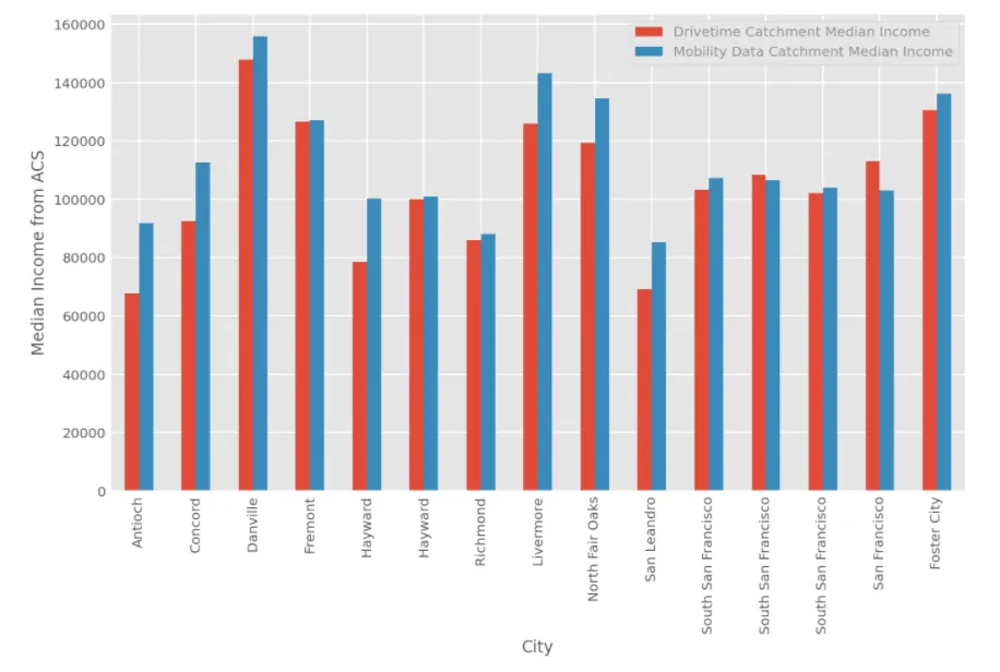
For some cities like Antioch and Hayward (one of the locations)  the difference is around 30%.

This would generally indicate that Costcos are located in neighborhoods that are poorer than the clientele who actually go to those Costcos. To keep this analysis simple  I only calculated median income differences. You can imagine the other kinds of demographic and economic disparities between the trade area we would find.

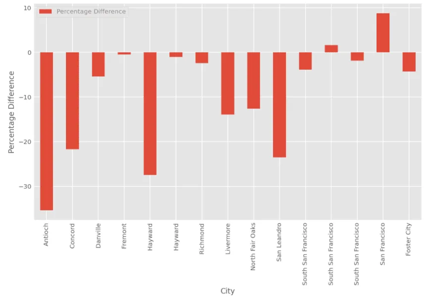
Here’s what these absolute value differences look like in Builder:

Competitive Intelligence using Human Mobility Data

Another valuable use of human mobility data is understanding who one’s competitors are. Drive times might give you one sense of who a location is competing with while mobility data might give another.

I imported Bay Area Walmarts and Targets into my map of Costcos to understand where they do and don’t compete with each other.

Let’s focus on one store to see this in action. The 15-minute drivetime for the Costcos located in Richmond  CA looks like this.

We might assume that those Targets to the south are the primary competitors of that Costco. But mobility data gives us a different sense of the trade area and the competitors.

We actually see how that specific visitors to Costco tend to come from El Cerrito and Richmond in the North and not as much from the Berkeley or Emeryville areas. Having a clear and accurate picture of who one’s competitors actually are is obviously important for so many business decisions.

Next Steps

Hopefully  this piece gave you a sense of the power of human mobility data for generating accurate trade areas. If you’re interested in learning more  both CARTO and SafeGraph offer generous free trials so that people and companies can test things out for themselves.

SafeGraph’s mobility data along with other location data streams can be viewed in our Data Observatory with SafeGraph also offering a helpful Python library for working with their data  which I used in my notebook.

If you’re interested in seeing more details on how analysis was performed  you can refer to these collab notebooks.

Want to learn more?

Sign up for an upcoming webinar with SafeGraph on this topic

This project has received funding from the European Union's Horizon 2020 research and innovation programme under grant agreement No 960401.