Map tiles: 5 examples to get started


Map tiles: 5 examples to get started


Efficiently visualizing large volumes of geospatial data is crucial in data analysis. However, this often requires compromising on either detail or scale, both of which limit the insights which can be derived.
Enter tilesets!
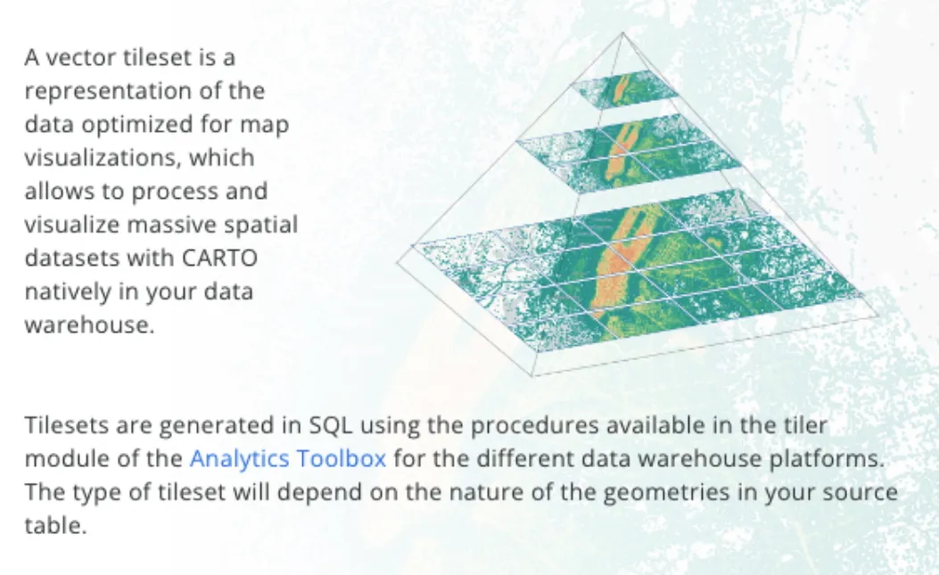
Tilesets revolutionize the spatial data rendering process. By dividing datasets into smaller, pre-rendered image tiles, tilesets enable faster loading, optimized bandwidth usage, and seamless navigation. With tilesets, users only load the necessary tiles for their zoom level and extent, ensuring a responsive and immersive map viewing experience.
Tilesets have been used by developers for a long time, however they have typically been difficult to build, requiring both engineering and geospatial skills. However… all of that is changing!
In this post, we’ll share a quick-start guide for creating tilesets followed by 5 fantastic examples of these in action to inspire you to start your tileset journey!
Before we start, you’ll need a CARTO account to follow these steps. If you don’t have one already, you can sign up for a free 14-day trial here.
💡 Did you know that you may already be working with tiles without realizing it? When your data exceeds the size limit for rendering as a GeoJSON (around 50MB), it is automatically rendered as a dynamic tileset. These tiles are generated on-the-fly during queries, requiring no extra effort from you. However, if you're working with exceptionally large datasets and experiencing suboptimal performance, it's recommended to generate your own tilesets for better results.
Follow the steps outlined below to create your first tileset!
- Navigate to the table you wish to transform into a tileset in the Data Explorer.
- Select Create a Tileset and choose a destination and output name.
- If you wish to query the data being input into the tileset, you can edit this in the SQL Editor, which you can turn on at the bottom of the wizard.
- In the Settings window, ensure the auto-detected geometry column is correct. You can also add in a description and modify the zoom levels your tileset will be rendered at.
- In the Attributes window, select which fields you wish to be included in the tileset.
- Finally, check all settings in the Confirmation window, and select Create! Depending on the complexity of the tileset, you may have to wait a short while for it to be created… and that’s it!
This process simply creates a tileset from a raw vector input. However, there are more advanced types of tilesets available which may be more beneficial to your use case:
- Aggregation Tilesets: instead of displaying individual points, these tilesets aggregate input information - such as count, sum or average - based on zoom level. This allows you to visualize trends and distributions at a level which is comprehensible for that zoom level. You’ll see some of these in action below!
- Spatial Index Tilesets: these tilesets leverage super-lightweight global grid systems like H3 and Quadbin to quickly render big data. Learn how to get started with Spatial Indexes with our free ebook.
If you would like to try out one of these more advanced processes - or would like more control over the process of creating a simple tileset - you can find a range of guides to help you get started in our Documentation.
Please note this process may differ depending on which cloud data warehouse you are using. Please see the guide specific to your data warehouse below:
Keep scrolling to see 5 fantastic examples of tilesets unlocking the power of big spatial data!
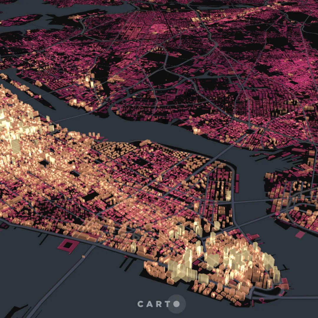
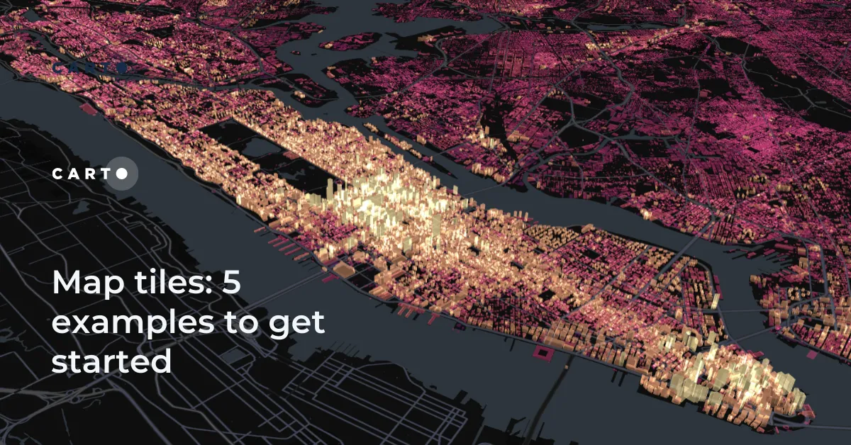
Remember the video earlier where we transformed a table into a tileset? This is the result! This map (open in full screen here) reveals building heights across the entirety of New York City.
The original dataset was sourced from NYC Open Data, with building footprints joined to a separate building heights dataset. The resulting table consisted of 1.1M individual buildings which equated to a 248.11 MB table - no wonder rendering was an issue!
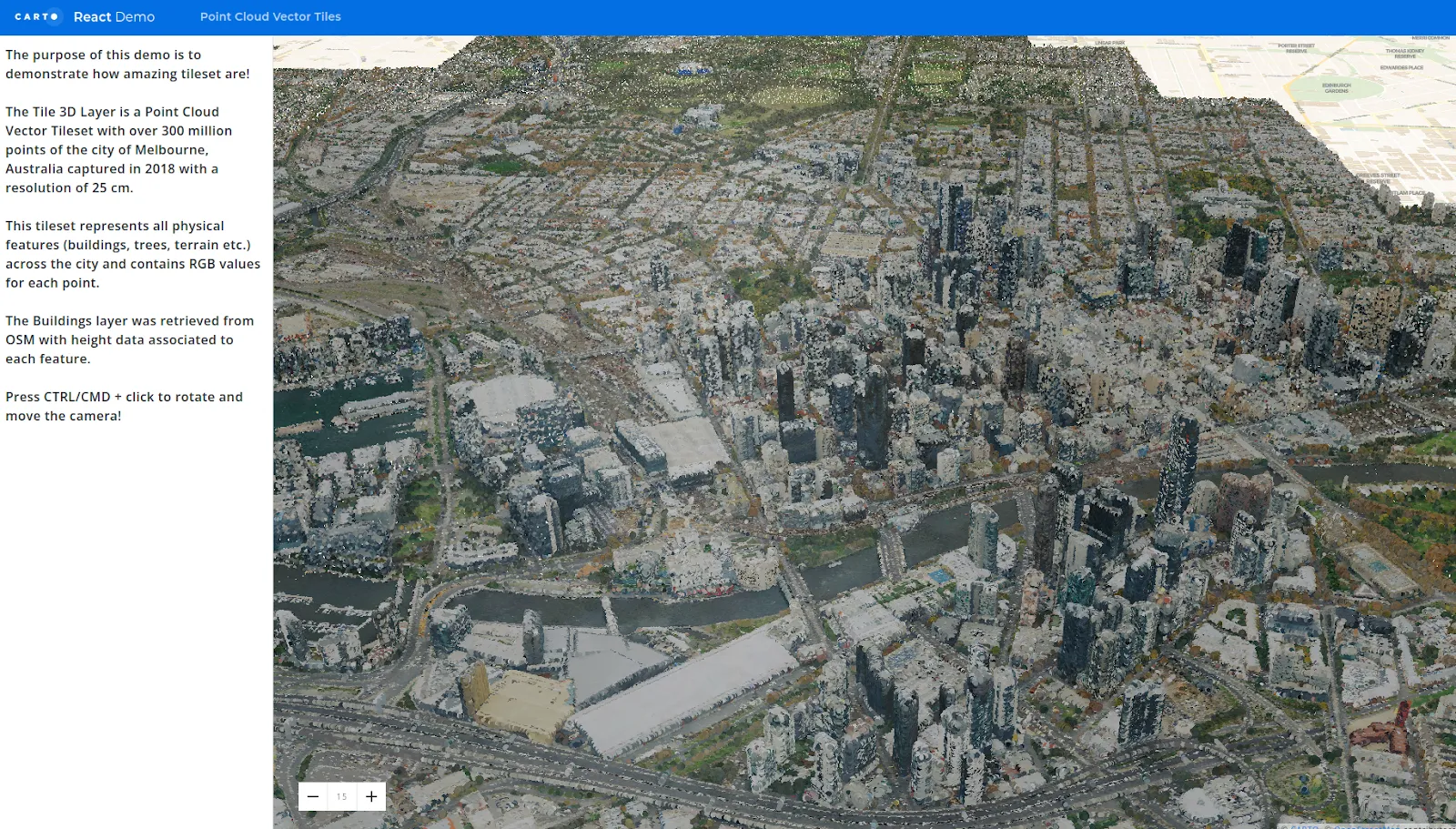
This map portrays Melbourne, Australia through a Point Cloud Vector Tileset.
The tileset contains a staggering 300 million points with an exceptionally detailed resolution of 25 cm. RGB values of each point are also included, allowing for a comprehensive representation of the city's physical features, including buildings, trees, and terrain.
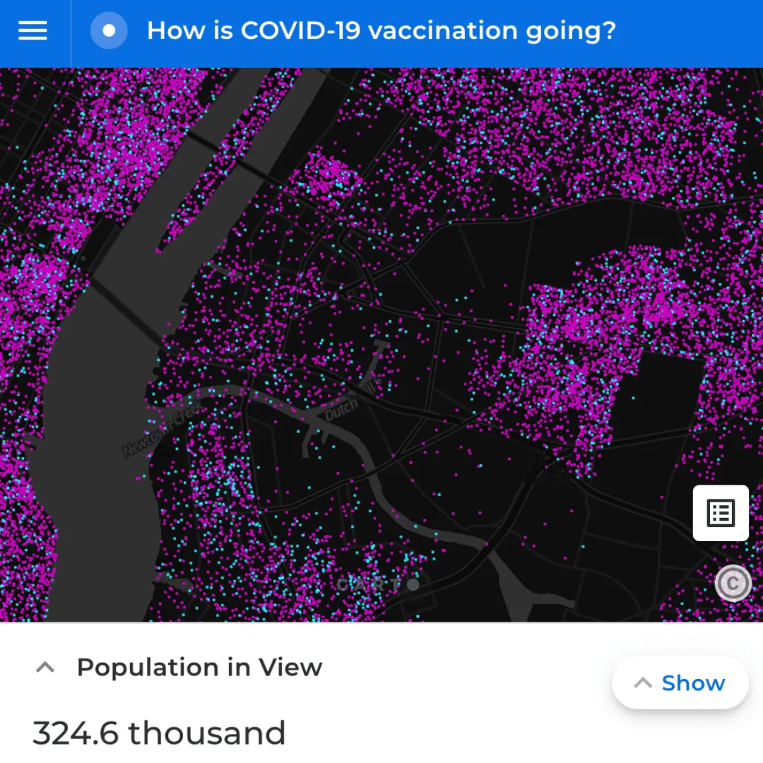
This example shows a tileset in which each of the approximately 330 million residents in the US is represented by means of a point. Each point is tagged with a vaccinated (blue) or non-vaccinated (purple) tag. This visualization enables us to depict at a glance how different parts of the country are progressing with the vaccination rollout.
This analysis leverages vaccination data from the Centers for Disease Control and Prevention as well as socio-demographic data from the CARTO Spatial Data Catalog. The SQL function ST_GENERATEPOINTS is used to generate a point representing each US citizen. Finally, the function CREATE_TILESET is used to convert this to the incredibly detailed tileset you can see above.
You can follow our tutorial for creating this map here.
OpenStreetMap - a global, crowdsourced dataset - contains 7.8 BILLION points making it an absolutely enormous dataset!
To be able to make sense of this dataset, the creator the CREATE_POINT_AGGREGATION_TILESET with darker areas representing more mapped features.
The source data for this has been accessed via the Google BigQuery Public Data Marketplace. If you want to leverage OpenStreetMap - often dubbed “The Wikipedia of Maps” - for your project, check out our ultimate guide to this dataset here!
In our final example, we showcase the contrast between rendering a layer with a table (left) versus a tileset (right), revealing a significant difference in performance.
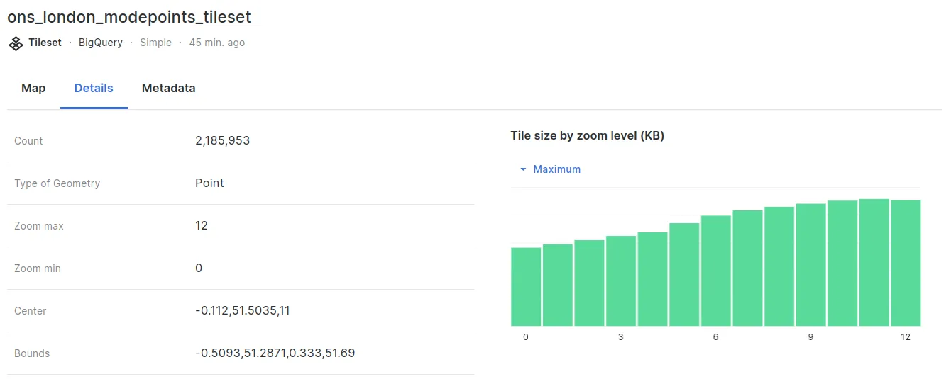
Both layers consist of approximately 2.2 million points, each representing a London resident’s mode of travel to work. This data was sourced from the UK’s Office for National Statistics and can be accessed here. It was then joined to the Output Areas geography, available via our Spatial Data Catalog.
The SQL function ST GENERATE POINTS was used to transform this into the dot density map you see here. You can learn how to create this type of map in this guide.
This example also highlights a significant difference in storage costs. The table version of this dataset weighs in at 128.28MB. Tilesets - however - are measured slightly differently.
Navigating to the Details section of your tileset in the Data Explorer will reveal the tile size by zoom level. At its maximum (zoom level 12), this tileset is only 453 KB - a fraction of the size of the table!
—
Ready to elevate your data visualizations with tilesets? Our platform enables you to generate tilesets natively directly inside your cloud data warehouse, no ETL needed! Sign up for a free 14-day trial!


.webp)


.webp)