Using BigQuery to build population maps for a vaccination app

Last week we published a spatial visualization to track the progress of the COVID-19 vaccination rollout in the US. It was very well received and many have asked us how this application was developed. In this follow-up post  we are going to take a deep-dive into the creation process covering all of the different components used across the CARTO platform and beyond.

The main tools we used for this analysis were:

• BigQuery: for analysis and data processing
• GitHub actions to extract and push the data to BigQuery
• CARTO's Spatial Analytics in BigQuery for the creation of random points and the TileSets
• CARTO for React to build the application and deploy it to Firebase.

Let's get started!

Sourcing the data

It is important to highlight that this is not personal data. We don't know which individuals are vaccinated or not  all we know is the percentage of vaccinated population by each county and state. From this data we can extrapolate the vaccine progress and create a simulation of individuals for the visualization.

Two main data sources were used as inputs into  our analytical approach:

1. Data from CDC on vaccination rollout numbers for each US state and county
2. Socio Demographic Population Data from the 2018 US Census available on BigQuery public-data project or as part of CARTO Data Observatory commercial datasets.

CDC data

As noted in last week's post  vaccination data from the CDC is utilized at both the state and county levels in our analysis  since coverage of data at the county level appears artificially low. In order for us to visualize this data within the app  it first needs to be loaded into BigQuery. This data ingestion phase is achieved using a combination of GitHub actions which can be represented by the diagram below.

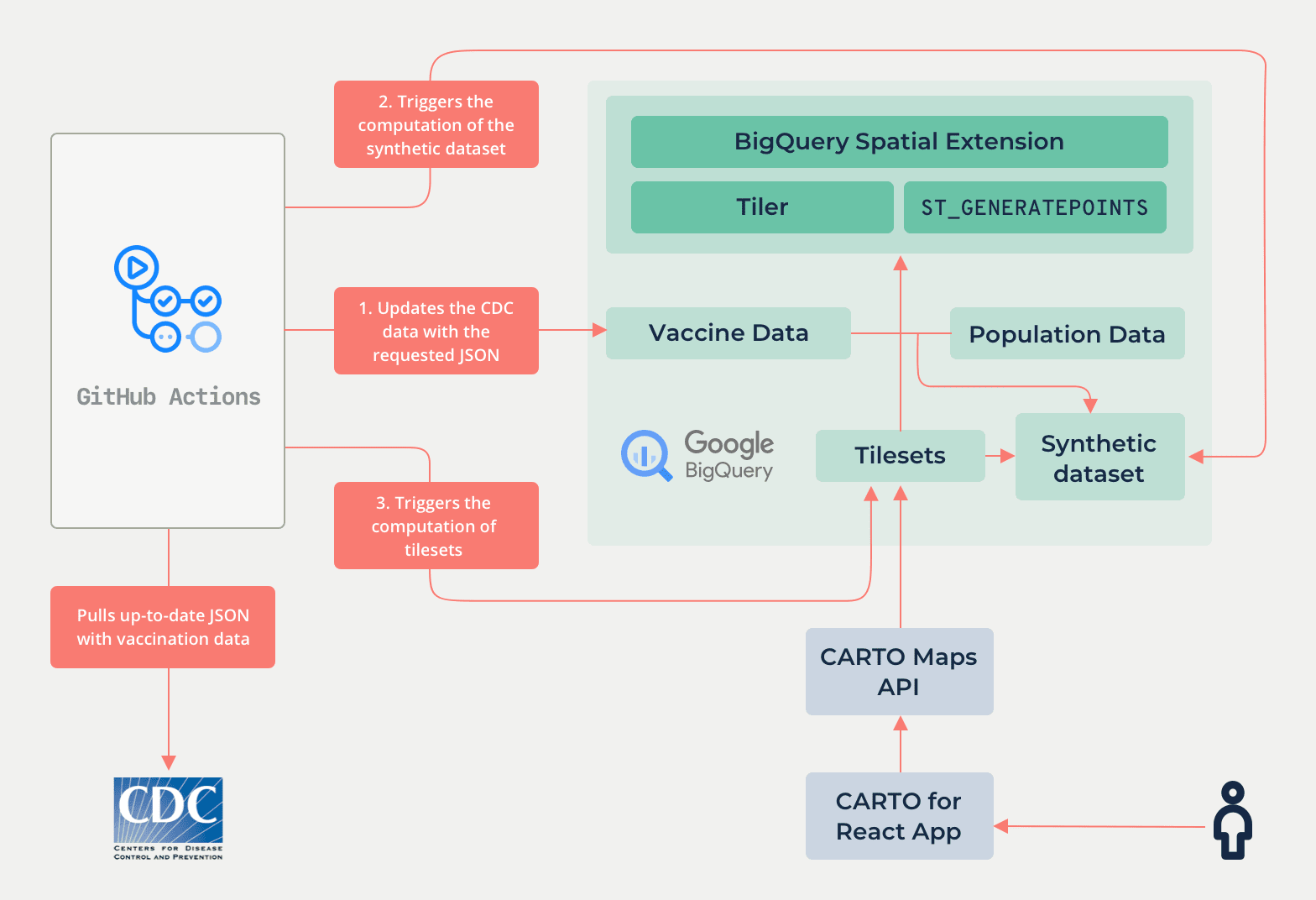
The script for sourcing the data runs every 2 hours automatically and checks if data has changed or not. If it has changed, then it uploads the new data to BigQuery and starts the processing to recreate the visualization.

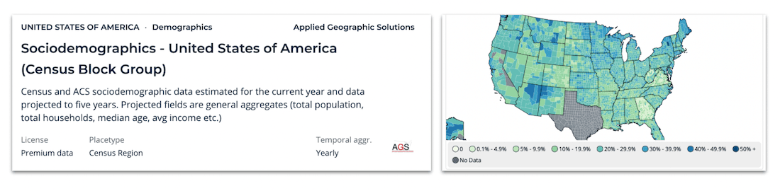
Socio demographic population data

Alongside the data from the CDC we have also utilized socio-demographic population data from the 2018 American Community Survey (an ongoing survey that provides vital information on a yearly basis about the US and its people), available for enrichment from our Data Observatory. This data set provides total population counts across the United States  expressed at the census block level.

We don't need to extract this data. The beauty of modern cloud data warehouse technology is that the data is already loaded in BigQuery by CARTO so you can just join to it.

Analyzing the data

Since the aim of the application is to visualize the progress of vaccination rollout at an individual level within each block group, we therefore need to calculate this data based upon the two input data sets.

We achieved this following a two-stage process. The first involves creating a synthetic dataset of the US population by generating a number of random points within each block group equal to its population.

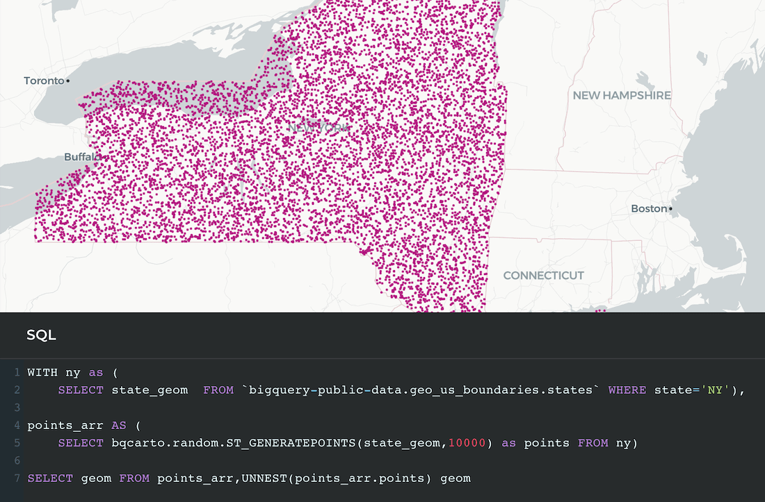
To do that  we pull on CARTO's Spatial Analytics in BigQuery we have for BigQuery, composed of a set of functions that can be run right inside BigQuery. The spatial function that we use for this task is ST_GENERATEPOINTS. The resulting dataset contains approximately 330M points, each of them representing a US inhabitant.

CARTO's Spatial Analytics in BigQuery works by enhancing BigQuery with further spatial capabilities coded as UDFs functions that can be run directly  for example:

SELECT bqcarto.random.ST_GENERATEPOINTS(state_geom 10000) as points FROM ny

The second stage consists of assigning a vaccination status attribute to each of these points  based on the vaccination percentage at the county level  as provided by the CDC. This is essentially a dasymetric mapping technique  where the CDC dataset at the county level is downscaled to block group level based on the distribution of the population.

Here is the SQL of the process detailed above:

CREATE OR REPLACE TABLE `cartobq.maps.covid19_vaccinated_usa_blockgroups_100pct` AS
    -- Extract the blockgroup geometry with its population
    WITH blockgroup_data AS (
        SELECT dem.total_pop AS population  geog.geom AS geom
        FROM `carto-do-public-data.usa_acs.demographics_sociodemographics_usa_blockgroup_2015_5yrs_20142018` dem
        INNER JOIN `carto-do-public-data.carto.geography_usa_blockgroup_2015` geog
        ON dem.geoid = geog.geoid
    ) 
    point_data AS (
        -- Vaccinated people section
        SELECT 
        bqcarto.random.ST_GENERATEPOINTS(
            blockgroup_data.geom  
            CAST(blockgroup_data.population * counties_vacc.Series_Complete_Pop_Pct * 0.01 AS INT64)) AS points  
        'true' AS vaccinated 
        FROM `bigquery-public-data.geo_us_boundaries.counties` counties
        INNER JOIN `cartobq.maps.cdc_raw_counties_data` counties_vacc 
        ON counties_vacc.FIPS = counties.county_fips_code
        INNER JOIN blockgroup_data 
        ON ST_CONTAINS(counties.county_geom  ST_CENTROID(blockgroup_data.geom))
        UNION ALL
        -- Non vaccinated people section
        SELECT 
        bqcarto.random.ST_GENERATEPOINTS(
            blockgroup_data.geom  
            CAST(blockgroup_data.population * (1.0 - counties_vacc.Series_Complete_Pop_Pct * 0.01) AS INT64)) points  
        'false' AS vaccinated 
        FROM `bigquery-public-data.geo_us_boundaries.counties` counties
        INNER JOIN `cartobq.maps.cdc_raw_counties_data` counties_vacc 
        ON counties_vacc.FIPS = counties.county_fips_code
        INNER JOIN blockgroup_data 
        ON ST_CONTAINS(counties.county_geom  ST_CENTROID(blockgroup_data.geom))
        UNION ALL
        -- There are several counties with unknown data
        SELECT 
        bqcarto.random.ST_GENERATEPOINTS(
            blockgroup_data.geom  
            CAST(blockgroup_data.population AS INT64)) points  
        'unknown' AS vaccinated 
        FROM `bigquery-public-data.geo_us_boundaries.counties` counties
        INNER JOIN `cartobq.maps.cdc_raw_counties_data` counties_vacc 
        ON counties_vacc.FIPS = counties.county_fips_code
        INNER JOIN blockgroup_data 
        ON ST_CONTAINS(counties.county_geom  ST_CENTROID(blockgroup_data.geom)) 
        AND counties_vacc.Series_Complete_Pop_Pct IS NULL
    )
    SELECT unnested_points AS geom  vaccinated  ROW_NUMBER() OVER() AS point_order
    FROM point_data  UNNEST(point_data.points) as unnested_points;

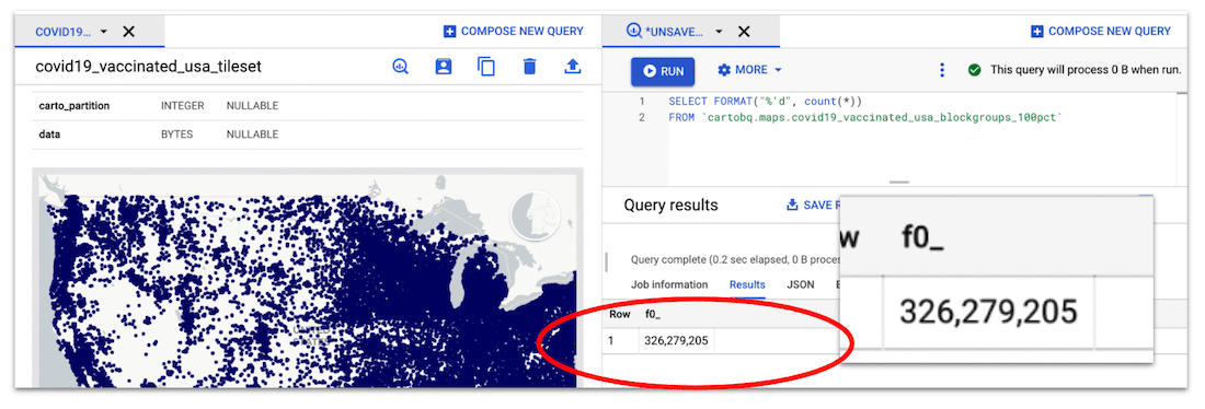
326 million records in a table as seen in BigQuery's new User Interface, with the CARTO Chrome Extension

Creating the tilesets

Visualizing 330 Million points on a map is not an easy task. Doing so effectively is even harder. Tilesets are the way to go when you are working with large data volumes  and CARTO provides a great way to generate tilesets directly from BigQuery. In this case we are using the CREATE_SIMPLE_TILESET function since we do not want to aggregate the data  we want to show every single dot on the map separately.

On the GitHub repository you can find the full query  and it goes like this:

CALL bqcarto.tiler.CREATE_SIMPLE_TILESET(
    SELECT vaccinated  geom FROM `cartobq.maps.covid19_vaccinated_usa_blockgroups_100pct `

) _a''' 
R'''`cartobq.maps.covid19_vaccinated_usa_tileset_temp`''' 
'''
    {
    ""zoom_min"": 0 
    ""zoom_max"": 15 
    ""max_tile_size_strategy"":""drop_fraction_as_needed"" 
    ""tile_feature_order"": ""point_order desc"" 
    ""properties"":{
        ""vaccinated"": ""String"" 
        ""point_order"":""Number""
    }
    }
'''
);

There is a lot going on in this query and it utilizes many capabilities of our BigQuery Tiler. A few of them include:

• We are using different sources based on the zoom level of the map. State data at higher zoom levels  county data at the lower levels. This way we can optimize performance and provide different visualizations at different zoom levels.
• You can see we are telling the tiler to drop_fraction_as_needed and we are setting a tile_feature_order. These 2 options provide a way to remove points to ensure the tiles on the tileset do not exceed a maximum size of 512kb. By doing so  we ensure the map looks great at any zoom level.
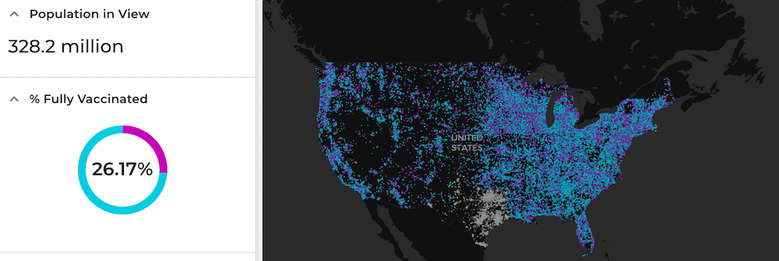
• If you look at this other tileset we generate  you can see that in order to have valid statistics at any zoom level  we create a secondary layer just for the data at a way lower resolution. This is key to ensure the widgets on the visualization display absolute values for the entire dataset  not just what is visible at a particular zoom level.

When all of this is done  and with some scripting  every 2 hours the source data gets updated, the synthetic dataset is recreated and finally the 2 tilesets are regenerated.

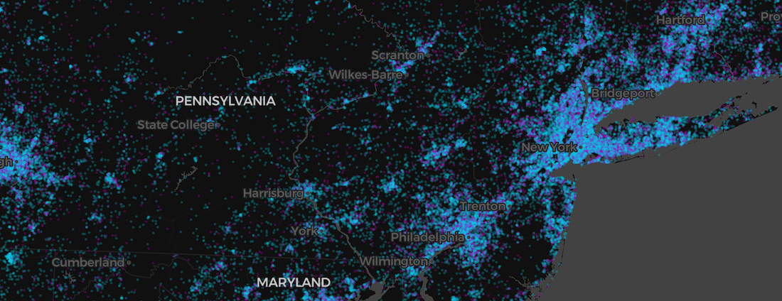
Aggregation tileset not visible which is used for powering widgets in the app.

Visualization Layer with the dots.

Building the app

We announced CARTO for React last month as the best way to develop Location Intelligence (LI) apps using the CARTO platform  React and deck.gl. By using the Create React App template we can dive straight into the creation of this app quickly and easily.

The deck.gl visualization is nested within the CARTO for React app and a number of innovative components have been brought together to create this application.

Check out the GitHub project for the app  there are instructions on how to create a similar app on the README.

One key part is the cartography for the visualization. We are using a pink and blue color following this great visualization by Ryan McCullough. In our case we make use of CARTO for deck.gl and therefore the styling of the map is done as follows. Checkout the colorCategory to specify the color based on the "vaccinated" property.

    return new CartoBQTilerLayer({
      id: VACCINES_LAYER_ID 
      data: source.data 
      credentials: source.credentials 
      getFillColor: colorCategories({
        attr: 'vaccinated' 
        domain: ['true'  'false'  'unknown'] 
        colors: [
          [204  0  194  255] 
          [0  210  230  180] 
          [200  200  200  110] 
        ] 
      }) 
      pointRadiusMinPixels: 1 
      pointRadiusMaxPixels: 12 
      pointRadiusScale: 1.9 
      getLineWidth: 0 
      ...cartoLayerProps 
    });
  }

Bringing it all together

Beyond the COVID-19 related insights this spatial application provides  it also demonstrates the relative ease of cloud-native spatial app development.

The components of the solution are integrated in such a way that it gives both developers and data scientists the functional capabilities to be able to ingest spatial data  carry out sophisticated analytical routines and also develop functionally rich user applications to visualize spatial data at scale.

Want to start using CARTO's Spatial Analytics in BigQuery?

Contact us to set up a meeting