On-demand last mile transportation: Real-time route optimization with Location Intelligence

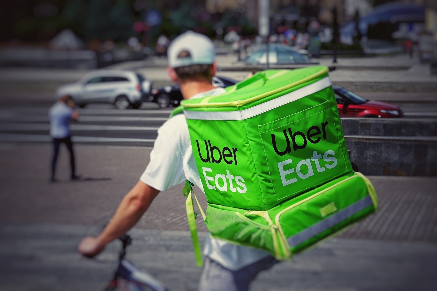
In recent years we have seen the emergence of numerous marketplace platforms connecting customers to a wide variety of products and services. Clear examples of this are Uber, Postmates, and Stuart that allow you to order pickup and delivery services of basically anything from a ride, to food, to even small parcels, and get it delivered in less than one or two hours.

Running this service efficiently is a challenge from a logistics point of view, and it is increasingly important in the face of fierce competition in the sector. Traditional logistics solutions are no longer suitable for planning such services due to the nature of the problem being very different from that of standard logistics companies. If we take a look at any regular third-party logistics (3PL) company, they normally accept next-day delivery orders until a certain cut-off time so that they have enough time to plan the next day’s routes. This is not the case for an on-demand service in which new orders have to be processed and assigned in (almost) real-time with no future information on the orders that may come in.

Both problems are notoriously difficult to solve, especially if we want to make sure we are operating optimally, or, at least, better than our competitors. This is where Spatial Data Science can make a difference as it allows us to build data models that simulate existing conditions, providing us insights on existing constraints, inefficient assignments, and much more.

Traditional vs on-demand last mile transportation problems

While both problems are difficult to solve, the complexity of each one can be found at very different stages. The traditional last mile transportation problem is a vehicle routing problem (VRP), a combinatorial optimization problem known for its complexity from an algorithmic design point of view as well as computationally. The clear advantage they have over the real-time on-demand transportation problem is that all the information about orders and driver availability is known beforehand, and normally a solution is not needed immediately. This makes it easier to find a near-optimal solution. There are several algorithms designed to solve this problem and several solvers with these algorithms implemented, both commercial and open source.

On the other hand, real-time on-demand transportation problems are smaller problems because there is less information available, but a response is needed immediately. Here we only know what happened up until the moment we check the state of the system, and most of it cannot be changed because it was already delivered. This can lead to very inefficient routing due to the lack of future information and the inability to change past decisions. Overcoming this narrow vision of the problem becomes the main challenge.

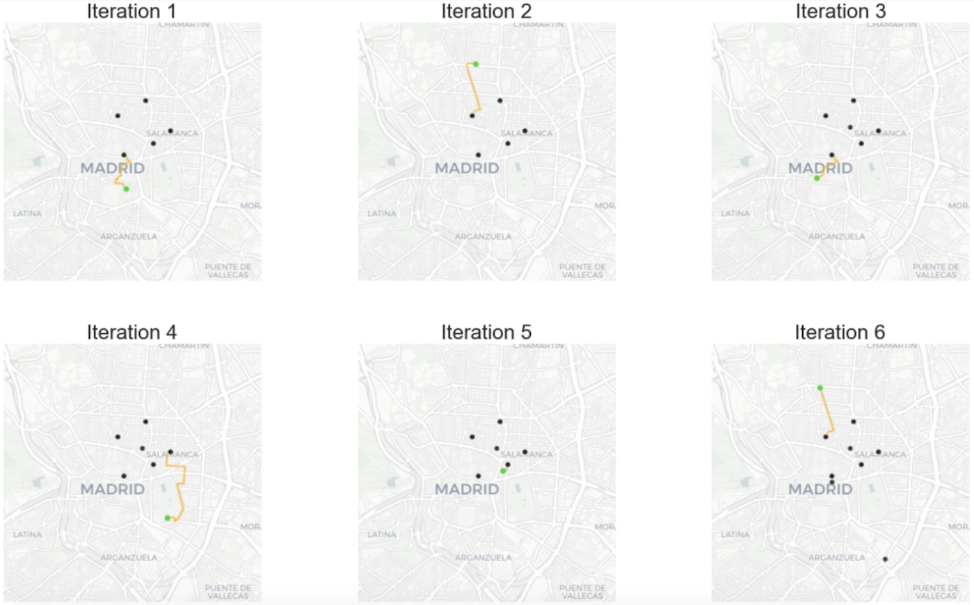
The following map is a good representation of this narrow vision, where we can only see the orders placed in every 3 minute time window. Once that time window is passed, we cannot change the assignments we made, and we do not have a vision of the orders that will come.

In logistics literature, there is consensus on how to overcome this narrow vision problem: adding flexibility to the decisions made, and trying to get as much future information as possible. The first point has to do with postponing decisions as much as possible and making decisions that can be easily undone or changed. The second one relates to the use of other Data Science techniques such as forecasting to broaden our vision.

This problem is harder to classify into a problem category because it will depend on the complexity of the service provided, and also on how far we want to go into optimizing our routes. It could go from a “simple” assignment problem (if we only need to consider the information related to a narrow time window) to a VRP (if we need to consider what drivers have done up until the current iteration of the algorithm).

The main challenge is then to be able to calculate all the required costs, and design an algorithm that can find a near-optimal solution in a matter of seconds. There can also be other challenges to overcome, such as calculating how many drivers we will need before we even start the day, what fleet we will need, or calculating the forecast for the following minutes/hours.

These big differences in the problem to be solved in both cases make it very hard, if not impossible, to adapt traditional logistics solutions to on-demand transportation problems.

Designing and improving an optimization algorithm

The following example shows a first step on how to apply optimization to solve the on-demand transportation problem, and the benefit obtained for doing so. Here’s a scenario for which we will apply two initial approaches to solve the problem.

The following assumptions are made to enhance the clarity of the presentation. However, bear in mind the problem can get more complicated depending on how far we want to go in optimizing how we function, and the requirements of the service provided as described later.

• The goal will be to minimize distances, and our main metric will be the total distance traveled. This could be easily changed to other criteria such as minimizing delivery time or the fleet needed  just to mention a few.
• Every order is independent of each other, i.e., they cannot be combined, hence why a rider will not be able to start an order until they finish the one they are currently delivering unless they are idle.
• Riders will not be assigned to a new order until they are idle.
• The type of fleet is the same for every rider.
• We will always have enough idle riders to assign to orders at each iteration of the algorithm. This  of course, will not be the case in real life and adds more complexity to the problem.

On the following map we can see orders received from 7:00 pm to 7:05 pm on a Thursday. We can see the pickup and delivery locations, the optimal routes calculated for each order, and the riders/drivers available who are idle or will be at some point within the time window. We are going to focus on this 5 minute time window to make it easier to show and compare results.

Step 1: Origin-Destination Matrix

In order to solve any routing problem we need to build a cost matrix representing the cost of going from place A to place B, or in the case presented here  the cost of assigning a rider located at point A to an order with pickup location at point B. In our example, this OD matrix will be the distances from riders’ locations to orders’ pickup locations.

In a previous post, we explained in detail how to build an OD matrix. This again is a harder challenge for the on-demand transportation problem because of the need to calculate this matrix in real-time.

Want to learn Postmates’ story? See it here!

Greedy algorithm

This is usually the first approach followed when solving this problem. This algorithm is activated every time an order is received and it searches the nearest idle rider and assigns the order to that rider. In this case, we are taking the nearest, but it could be any other criteria to be optimized depending on the service provided or the business goals.

This algorithm is widely used because it is very easy to implement, and to understand and analyze its results. In addition, when launching a new business  customer experience is usually one of the main metrics, so it makes sense to want to process each order as soon as possible. However, this does not necessarily mean that the customer will always be served faster.

After solving the problem with this algorithm we get a total distance of 181.67 km traveled by riders from their starting locations to the pickup locations.

In the following figure we can see the first six steps performed by the algorithm plotted using CARTOframes where black points are the locations of idle riders, and green points are the orders’ pickup locations. This visualization is very powerful because it can help quickly identify inefficiencies in our algorithm.

Batch assignment algorithm

As mentioned before, a key factor to improve the assignments is to add as much information and flexibility as possible. One option to broaden our vision and get more information would be to postpone the order assignment and run the algorithm every n minutes. The more we can postpone it the better  because we will have more information.

The following figure shows the number of orders received every minute.

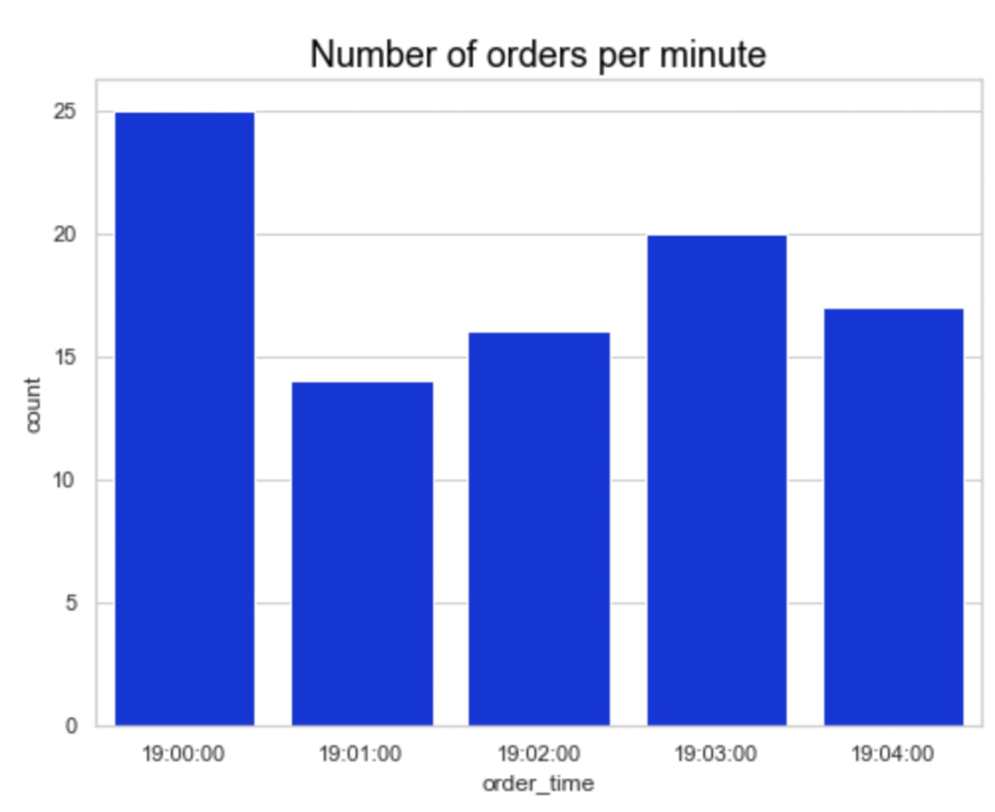
Running the algorithm every minute means that an order will have to wait (at most) one minute to be processed, which initially should not have a significant impact on customer experience. In fact, we’ll see that some orders will get delivered even before.

The algorithm will be activated every minute, and it will consider all the orders received in the last minute and assign them. This means it will have more than one order to assign. In order to make the most of all the information we have, we will solve this as an assignment problem.

There are specific algorithms designed for this problem such as the Hungarian algorithm. Normally, these algorithms are designed for very specific cases of the problem and it is hard to evolve them when the problem starts to require complex features. That is why we will solve it using Linear Programming  or more specifically Integer Linear Programming. This technique will allow us to adapt to future changes or adding more complexity to the problem.

{::options parse_block_html="true" /}

### Linear Programming in a nutshellA typical linear program looks as follows:$$max \text{  } c^Tx$$$$\text{s.t.  } Ax \leq b$$$$x \geq 0$$$$A \in \mathbb{R}^{mxn}  x\in \mathbb{R}^n  c\in \mathbb{R}^n  b\in \mathbb{R}^m$$And it has the following components:- **Decision variables** ($$x\in \mathbb{R}^n$$)
Decision variables represent the decisions that need to be made and that will lead to an optimal plan. The decision variables of our problem will be the ones indicating which rider is assigned to which order. A solution is achieved once every variable is instantiated to one single value.- **Objective function** ($$max \text{  } c^Tx$$)
The objective function is the measurement/metric that will allow us to determine objectively whether one solution is better than another. In this case, it will be the sum of all the distances made by the riders.- **Constraints**
Constraints define what solutions are feasible from different points of view. We can have, for example, physical constraints (a rider cannot deliver more than one order at once), and business constraints (best customer’s orders are served by best riders). Both the objective function and the constraints must be linear expressions for the model to be considered a linear program.The most well known algorithm for solving linear programming models is the [Simplex algorithm](https://en.wikipedia.org/wiki/Simplex_algorithm) or any of its variations. [Interior point algorithms](https://en.wikipedia.org/wiki/Interior-point_method) are also widely used. There are quite a few solvers with these algorithms implemented, both commercial and open source. These solvers usually combine the Simplex or interior point algorithms with presolving and heuristics techniques. The strength of these techniques is what usually what makes a good solver.An **Integer Linear Program (ILP)** is a linear program in which all variables are integer variables. In our problem, they are all binary variables.

### On-demand transportation assignment model $$\textbf{Indices}$$ $$i=\{1  2  . . .  I\} \text{   orders}$$$$j=\{1  2  . . .  J\} \text{   riders}$$

$$\textbf{Parameters}$$$$d_{ij}: $$ distance from rider j‘s starting location to order i‘s pickup location

$$\textbf{Variables}$$$$X_{ij}: $$ binary variable indicating whether order i gets assigned to rider j

$$\textbf{Objective function}$$$$min \sum_{ij}d_{ij}X_{ij}$$

$$\textbf{Constraints}$$$$(1) $$ Every rider is assigned to at most one order$$\sum_iX_{ij}\leq 1  \forall j$$

$$(2) $$ Every order is assigned to at most one rider$$ \sum_j X_{ij} \leq 1  \forall i$$

$$(3) $$ Assign as many orders as possible$$\sum_{ij}X_{ij} = min\{I  J\}$$

$$(4) $$ Natural constraints$$X_{ij} \in \{0  1\}  \forall i j$$

After solving the problem with this Batch Assignment algorithm we get a total distance traveled of 159.10 km  i.e., we get a 13% improvement in our goal metric.

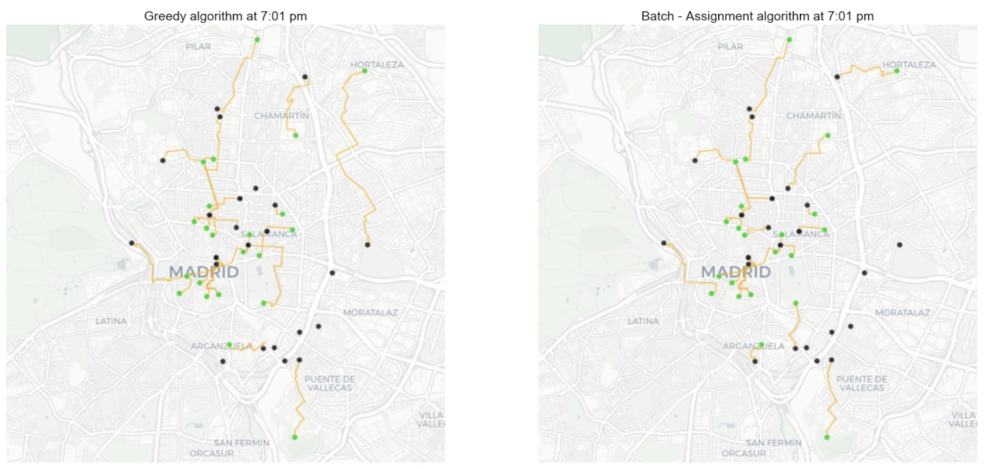
If we compare the assignments done on the orders received in the first minute (from 7:00 to 7:01 pm) with both algorithms we can see some big differences. For example, if we look at the north-east part of the map, we can see a very inefficient assignment done with the greedy algorithm that has a much more efficient assignment with the batch assignment algorithm. This is thanks to having more information by postponing when assignments are done.

Here again, being able to visualize the decisions made by both algorithms is very powerful:

Next steps

The previous two algorithms are just the first natural steps that are normally followed when faced with this problem. However, the complexity of the problem usually asks for more steps.

As mentioned above, broadening the information available at each iteration of the problem is essential. One very useful step would be to make assignments considering what could happen in the following 30 to 60 minutes (or even more time depending on the length of the services). It would be very helpful to have some forecast of where the demand will be so as to avoid assignments that will move riders far from the higher demand areas. This could easily be incorporated into the Batch Assignment model by identifying which riders should not be assigned to orders with delivery location far from the higher demand areas. In addition, this information could be made available to riders so that they know where they should move when idle to be sure they’re assigned more orders.

The following map shows where the demand is expected to happen an hour from now, together with the idle riders. Depending on how far they are from the higher expected demand areas, they will be given a different priority to be assigned.

Apart from this, there are other improvements that would lead to more efficient and higher quality assignments. These improvements would strongly depend on the type of service provided.

• Optimization criteria. In our example we took distance as the metric to be optimized. However, we might add extra criteria, always bearing in mind that costs have to be calculated at every iteration of the algorithm. Some examples could be:
• Time
• Utilization. This is especially important for companies where the fleet is expensive to acquire and/or maintain.
• Customer and rider experience.
• Matching the quality of the customer in terms of the frequency of use of the service  and the quality of the rider based on the customer’s opinions and efficiency in delivery.
• Combining orders (e.g. Uber pool)
• Create larger batches by postponing the assignment as much as possible. For example, for delivering small parcels 5 minutes may be fine.

Incorporating these criteria into our model is a complex task from an algorithmic point of view. Being able to visualize the steps and decisions made by the different algorithms we test is a very powerful tool for a very time-consuming task. Here CARTOframes can be of enormous help.

Special thanks to Mamata Akella, CARTO's Head of Cartography, for her support in the creation of the maps in this post.