How to build a revenue prediction model with CARTO & BigQuery

Sales forecasting and revenue prediction have become increasingly important to retailers during the past two years as store owners have had to rapidly react to evolving consumer behaviors.

For example, understanding what consumers will buy, how much, and when can be used by retailers to optimize revenue by avoiding over or under-stocking key product lines. Historical sales data has been traditionally used to create such a forecast but retailers also need to consider the location aspect within their analysis, especially when it comes to decisions around site selection.

This year, retailers in the US will open more stores than they close for the first time since 2017 (source) with ‘retail’s recovery going faster than anyone imagined’.

Trends identified by our own Black Friday analysis also illustrate a recovery period between 2020 and 2021 but crucially showed that people do not seem to be traveling as far to shop. Being able to predict the revenue potential for different locations is critical for an optimal site selection strategy, allowing retailers to reduce the time and effort required to pinpoint the best store locations for their business.

In this blogpost we will showcase how to use CARTO's Analytics Toolbox for BigQuery to train a spatial model to predict annual store revenues across a territory.

The recently announced CARTO Spatial Extension for BigQuery is a complete redevelopment of our leading Location Intelligence platform. One of the key components of this platform is the Analytics Toolbox  which provides a complete framework of analysis capabilities to perform spatial analytics in SQL, computed natively in the leading cloud data warehouse platforms. Our implementation for BigQuery enables users of such a platform to have a fully cloud native GIS and Spatial Data Science experience while keeping the benefits around privacy, compliance, scalability, and lower costs that their data warehouse brings.

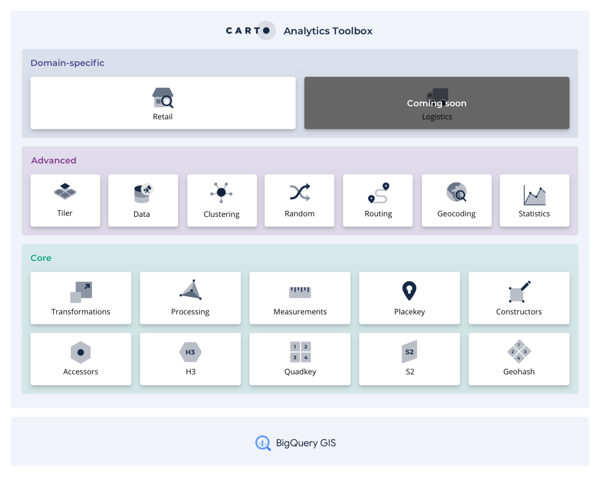
The analysis routines in the Analytics Toolbox cover a broad range of spatial analytics use-cases and are organized into a series of modules (data, clustering, statistics  etc.) based on the functionality that they offer. Today, we are happy to announce the availability of a new domain-specific module to solve geospatial analytics for the retail sector  starting with Revenue Prediction.

Revenue Prediction with the Analytics Toolbox

In order to carry out revenue prediction analysis we have implemented three new procedures into the Analytics Toolbox that leverage the scalability and computational efficiency of spatial indexes and cover all the necessary steps to solve this use-case  end-to-end: data prep  model training  and prediction.

• BUILD_REVENUE_MODEL_DATA: as a first step in the revenue prediction workflow, this procedure prepares the data to build the revenue prediction model, which will be used in both the training and prediction phases. As a result, the area of interest for the analysis is polyfilled using either H3 or quadkey spatial indexes and enriched with features from both Data Observatory datasets and user's first party data (including store revenue) in order to characterize it.
• BUILD_REVENUE_MODEL: builds the predictive model from the input data (i.e.  output from the previous step), the advanced configuration options, and computes the model's and features' statistics (mean absolute error  feature importance  etc.).
• PREDICT_REVENUE_AVERAGE: the final procedure in the workflow that predicts the potential revenue of a new store to be located in a particular area.

It is important to note that these procedures are leveraging other routines from our Analytics Toolbox concurrently such as MORANS_I_H3  ENRICH_GRID and DATAOBS_ENRICH_GRID. You can learn more about enriching spatial data here.

For the purpose of this case study we are going to use the publicly available Iowa Liquor Sales data, which provides spirits purchase information at store level for Iowa Class "E" liquor licensees by product and date of purchase from January 1st 2012 to present time. In particular  we are going to train our predictive model with the revenue data of the 135 stores that appear under the brand "Hy-Vee"  computed as the aggregate sales data at yearly level. These stores are used as a reference and the model is built using their locations and revenues as inputs. All other liquor stores will be considered Hy-Vee's competitors. Then  we are going to simulate the scenario in which we want to predict the revenue of a new Hy-Vee store located anywhere in the state of Iowa.

Additionally  in order to train the revenue prediction model we are going to enrich the store revenue data with location-aware context, specifically with variables from CARTO's Spatial Features dataset at H3 Resolution 8 level  available via our Data Observatory.

Data Preparation

The first step of the Revenue Prediction analysis workflow consists in preparing the data that will be used to both train the model and run predictions. The area of interest for our particular use-case is the entire state of Iowa in the US  which we are going to analyze using a H3 grid of resolution 6. The H3 grid cells within this area will be enriched with the number of Hy-Vee's stores in each grid cell  their average annual revenue  and the number of competitor's stores.

Moreover  this H3 grid will be enriched with the total population and number of POIs of different categories, in particular, retail, financial, food & drinks, leisure  transportation and tourism. This data is extracted from CARTO's Spatial Features dataset  available via our Data Observatory. For this enrichment  the value of these variables for each particular grid cell and their neighboring cells  defined as those within a KRING of size 2  will be taken into account. The values at the neighboring cells will be scaled according to a configurable decay function  in this case a uniform function  with the objective of giving less weight to those cells that are further away from the origin cell.

CALL `carto-un`.carto.BUILD_REVENUE_MODEL_DATA(
  -- Stores: revenue  store  geom
  '''
  SELECT store_name as store, store_location as geom,  sum(sale_dollars) as revenue FROM
 `bigquery-public-data.iowa_liquor_sales.sales`
  where store_name like "%Hy-Vee%" and EXTRACT(YEAR FROM date)=2019
  group by store_name
  ''', 
  -- Store variables
  NULL, 
  -- Competitors: competitor,  geom
  '''
  SELECT store_name as competitor, store_location as geom as geom FROM
 `bigquery-public-data.iowa_liquor_sales.sales`
  where store_name not like "%Hy-Vee%" and EXTRACT(YEAR FROM date)=2019
  group by store_name
  ''', 
  -- Area of interest: geom
  '''
  SELECT state_geom AS geom
  FROM `bigquery-public-data.geo_us_boundaries.states`
  WHERE state_name='Iowa'
  ''', 
  -- Grid params: grid type and level
  'h3',  6, 
  -- Decay params: kring size and decay function
  2 , '', 
  -- Data Observatory enrichment
  [("population_f5b8d177",  'sum'),  ("retail_21cb1815", 'sum'), ("financial_9b8bb507", 'sum'), ("food_drink_bd2ef444", 'sum'), ("leisure_16da1bd6", 'sum'), 
  ("transportation_63a2617a", 'sum'), ("tourism_fc201498", 'sum')], 
  '<my-dataobs-project>.<my-dataobs-dataset>', 
  -- Custom data enrichment
  NULL,  NULL, 
  -- Output destination prefix
  'cartobq.docs.revenue_prediction_iowa'
);

Where <my-dataobs-project>.<my-dataobs-dataset> specifies the location of the user’s Data Observatory subscriptions in BigQuery.

In the map below, we showcase Hy-Vee's stores styled by their yearly revenue and the enriched H3 grid that we will use to train and run the model  styled by the weighted population at each cell (i.e.  considering also their neighbors as explained previously).

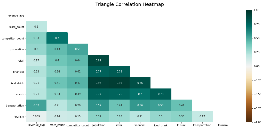
Now that our training data is ready  we can perform a simple correlation analysis to understand the relationship between all pairs of variables. In the diagram below  where one-to-one correlations are shown  we can identify a strong relationship between food & drink POIs with both population and retail POIs. This is expected as restaurants  coffee shops  etc. tend to be located in highly populated areas. In addition  a significant relationship is observed for the existing store count and number of competitors variables. This means that the more stores are present in a particular grid cell  the more competitor stores there are  which is expected from a business perspective. Finally  we can highlight that the lowest correlated variables are the number of tourism POIs and the annual revenue.

Model Training

Now that we have the data prepared, we can run the second procedure  BUILD_REVENUE_MODEL  in order to build and train the predictive model.

CALL `carto-un`.carto.BUILD_REVENUE_MODEL(
   -- Model data
   'cartobq.docs.revenue_prediction_iowa_revenue_model_data', 
   -- Options
   '{"MAX_ITERATIONS": 20 , "MAX_TREE_DEPTH":3}', 
   -- Output destination prefix
   'cartobq.docs.revenue_prediction_iowa
'
);

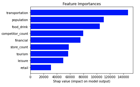
The outputs of this procedure are the trained model to be used in the revenue prediction  a SHAP table containing the list of the features and their attribution to the model  a model stats table (e.g.  mean error  variance  etc.)  and finally a table with the model's feature importance.

Finally  in order to showcase the performance of our predictive model we use the following metrics  R-square and Mean Absolute Percentage Error (MAPE). As can be seen  the model is able to explain 87% of the variance  and the average prediction error is ±25%

‍

Revenue Prediction

To predict the revenue of a new store located in any of the H3 grid cells within our area of interest (the state of Iowa), we can simply run the PREDICT_REVENUE_AVERAGE procedure  providing as inputs the corresponding cell ID  the model data (output of the BUILD_REVENUE_MODEL_DATA procedure) and the revenue model (output of the BUILD_REVENUE_MODEL procedure).

CALL `carto-un`.carto.PREDICT_REVENUE_AVERAGE(
   '862674467ffffff', 
   'cartobq.docs.revenue_prediction_iowa_revenue_model', 
   'cartobq.docs.revenue_prediction_iowa_revenue_model_data', 
   NULL, 
   NULL,
);

In the map below we can see the revenue predictions for a set of locations within Iowa where there were previously no existing stores  along with the annual revenue of the existing stores and the location of the competitors considered for this analysis.

The prediction results for all grid cells within Iowa can be found in the table cartobq.docs.revenue_prediction_iowa_all_predictions.

This is just the first retail-specific use case that we can solve with our Analytics Toolbox for BigQuery. In the coming months we will be adding other advanced use cases to the Retail module such as Twin Area Analysis, Whitespace Analysis  and Commercial Hotspot Analysis.

The revenue prediction procedures are now available from the Analytics Toolbox for BigQuery and can be run directly from the BigQuery console or from your SQL or Python Notebooks using the BigQuery client. Additionally  they will soon power the revenue prediction analysis engine integrated in CARTO's Site Selection application.  

The Analytics Toolbox for BigQuery is a component of our cloud native Location Intelligence platform. To access, sign up for a free trial or contact our team of experts for a personalized demo.

Want to get started?

Sign up for a free 14-day trial

This project has received funding from the European Union's Horizon 2020 research and innovation programme under grant agreement No 960401.