New to CARTO? Try these 5 things first!


So you’re ready to start your CARTO journey - congratulations!
If you’re new to CARTO and not sure where to start, you’re in the right place! In this post, we'll run through the first five things you should try.
Not got an account? That’s easily solved! Sign up for a free 14-day trial account here (which is exactly the same as a non-trial account, just… well, it only lasts for 14 days!).
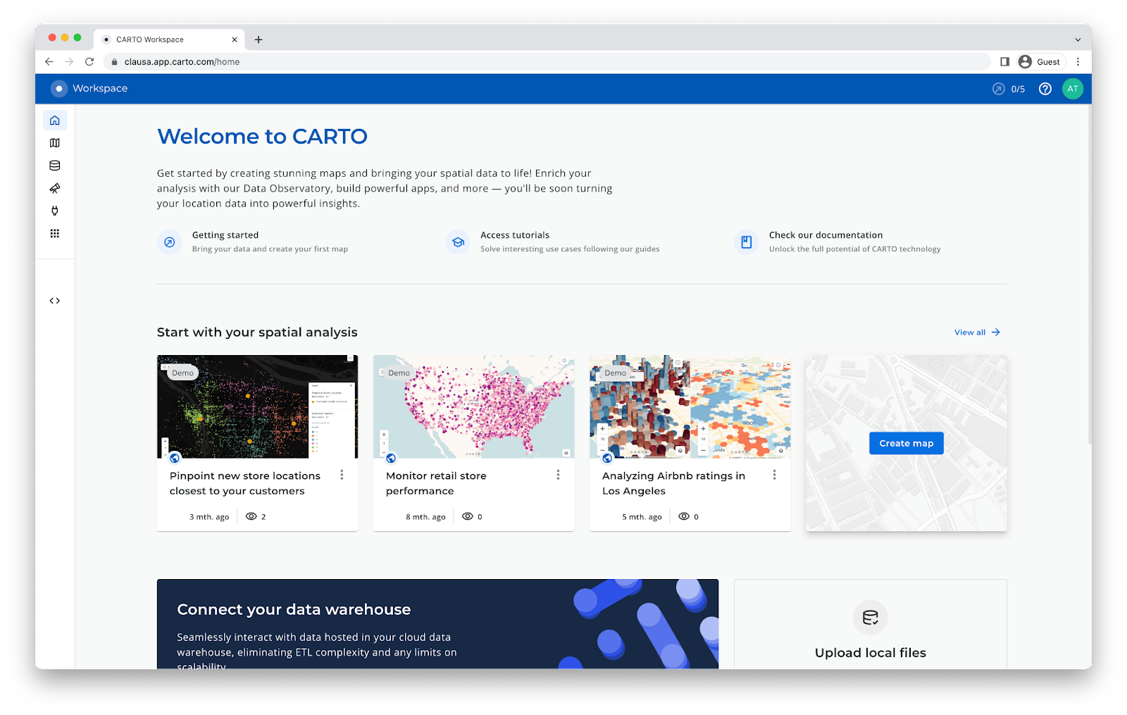
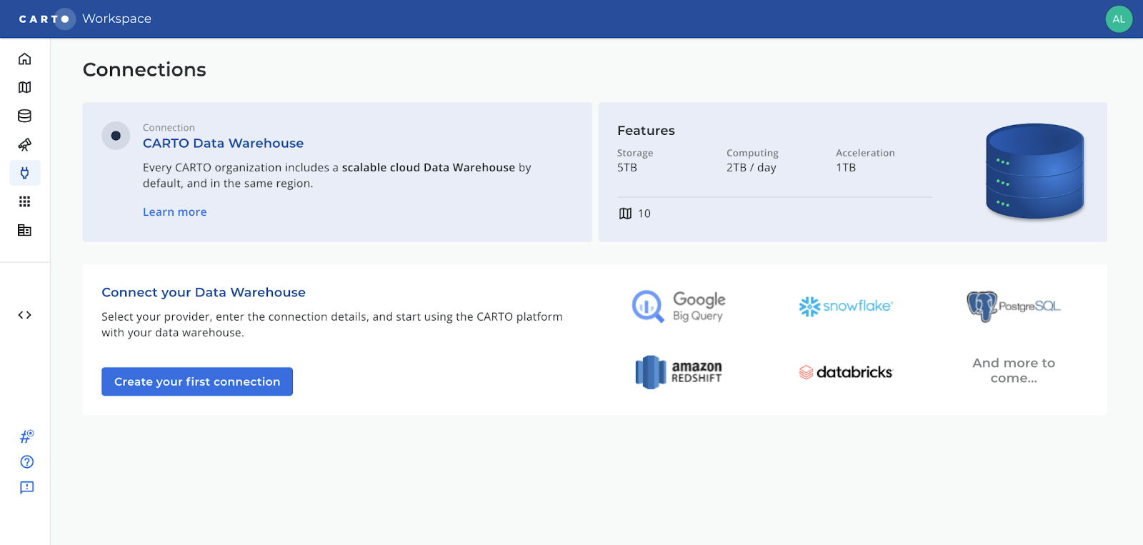
Once set up, head to app.carto.com and login. You should see a window that looks a little something like the one below. This is your CARTO Workspace and will be the hub for all things CARTO. No software download, no slow install - just login and go! While you're onboarding, from the workspace home you'll be able to follow the Getting started steps (beneath "Welcome to CARTO") to help you get used to the CARTO platform.
So… shall we?
Step 1: Connect your data
If you aren’t already aware, one of the things that makes CARTO special is that it’s entirely cloud-native. That means that all of your processing and analytics happens directly inside your data warehouse. Your data never has to leave your data warehouse, and you don’t have to worry about long and complex ETL processes, or the painful data governance that comes with storing data across multiple locations.
So - the first thing you need to do? Connect to your data warehouse!
- Hover over the panel on the left of your workspace and select Connections
- Select New Connection
- Choose your data warehouse provider
- Enter the credentials of your data warehouse
- Connect!
Back on the left hand side of the screen, select Data Explorer > Connections. You’ll see you can now access all of your data - it’s that easy!
Help - I don’t have a Cloud Data Warehouse!
Not a problem! Every CARTO user is provided with access to the CARTO Data Warehouse connection. This will grant you access to both a private and organisation-wide cloud storage and computing space, the amount of which will depend on your subscription plan. You can also import data from URLs or local files into this location, as well as access a range of demo tables and tile sets to work with.
However, to really scale your analytics we recommend setting up spatial infrastructure on the cloud. We have a host of resources to help you with this, such as this step-by-step guide to migrating from postgreSQL to Snowflake.
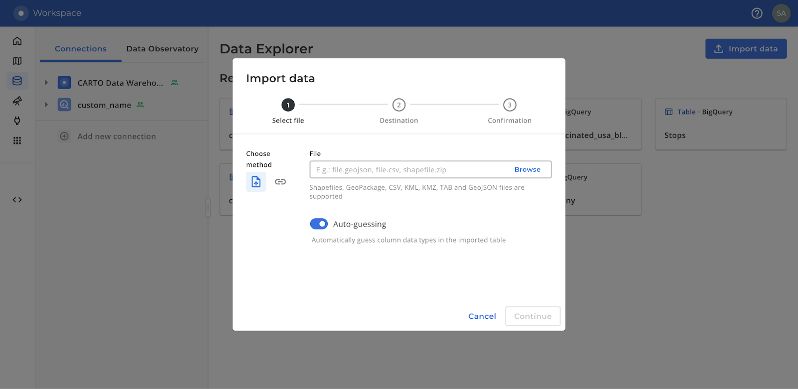
You can also use the CARTO UI to import spatial data directly to your data warehouse. From the Data Explorer you can find the Import wizard to the top right of the Data Explorer window (see below).
Step 2: Create a map
Now let’s get straight to the fun stuff - let’s make a map! Check out the video below or keep reading for a quick-start guide.
- In the Maps tab of the CARTO Workspace, select + New Map to open CARTO Builder - your tool for building maps and dashboards at a huge scale.
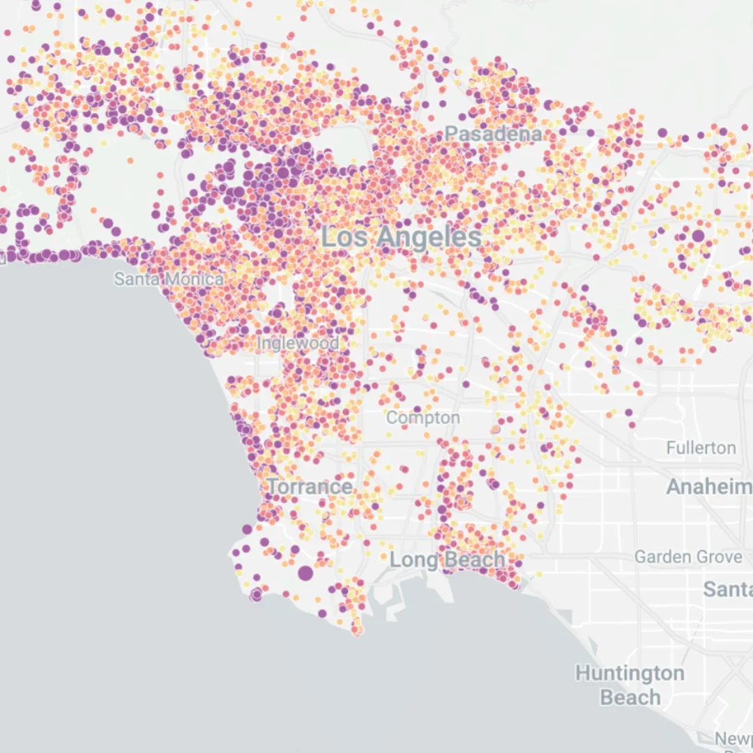
- First - let's add some data! In the bottom-left of the screen, you'll see the Sources panel. Select Add source from > Data Explorer and navigate to a table of your choosing. We're going to head to the CARTO Data Warehouse > demo tables and add the Los Angeles Airbnb demo table. Select Add Source - and your layer will be added to your map!
- In Layers panel on the left of the window, select the Layer you've just added (probably called Layer 1) to open the layer options. Select the three dots next to the name to rename it, then explore the layer styling options. For instance, we've added a white stroke to our Airbnb locations, and set both the fill color and radius to be determined by the price.
- At the top left of the window, switch from the Layer to the Widget tab. This is where you can add all sorts of dynamic graphical elements to help your user explore the map. We've added one widget showing the total number of Airbnbs and one showing a histogram of property prices. Check out how the widgets update as you explore the map - you can even interact with the widgets to filter your data!
- Switch from the Widget tab to Interactions (just to the right) and enable interactions for your layer. Select the interaction style and choose which fields to include in the interactions. You can change the field format and name here - or optionally switch to HTML to fully customize your pop-up, even adding automatically generated Google Streetview images (check out our guide to this here!).
Open this map in full screen here.
This is just the tip of the iceberg when it comes to CARTO Builder's capabilities - try exploring some of the other options, including 3D, split-screens and custom basemaps!
Once you’re happy with your visualization make sure to give it a name (top left of the screen), then hit the share button (the padlock icon to the top-right of the screen) and select who can view your map (private, public, password-protected or organization-only) - you’ll now be given a link which you can use to show the world your hard work!
Make sure you head to the Data Visualization section of the CARTO Academy for a wide range of tutorials to help you to start crafting powerful maps at scale!
Step 3: Subscribe to some data
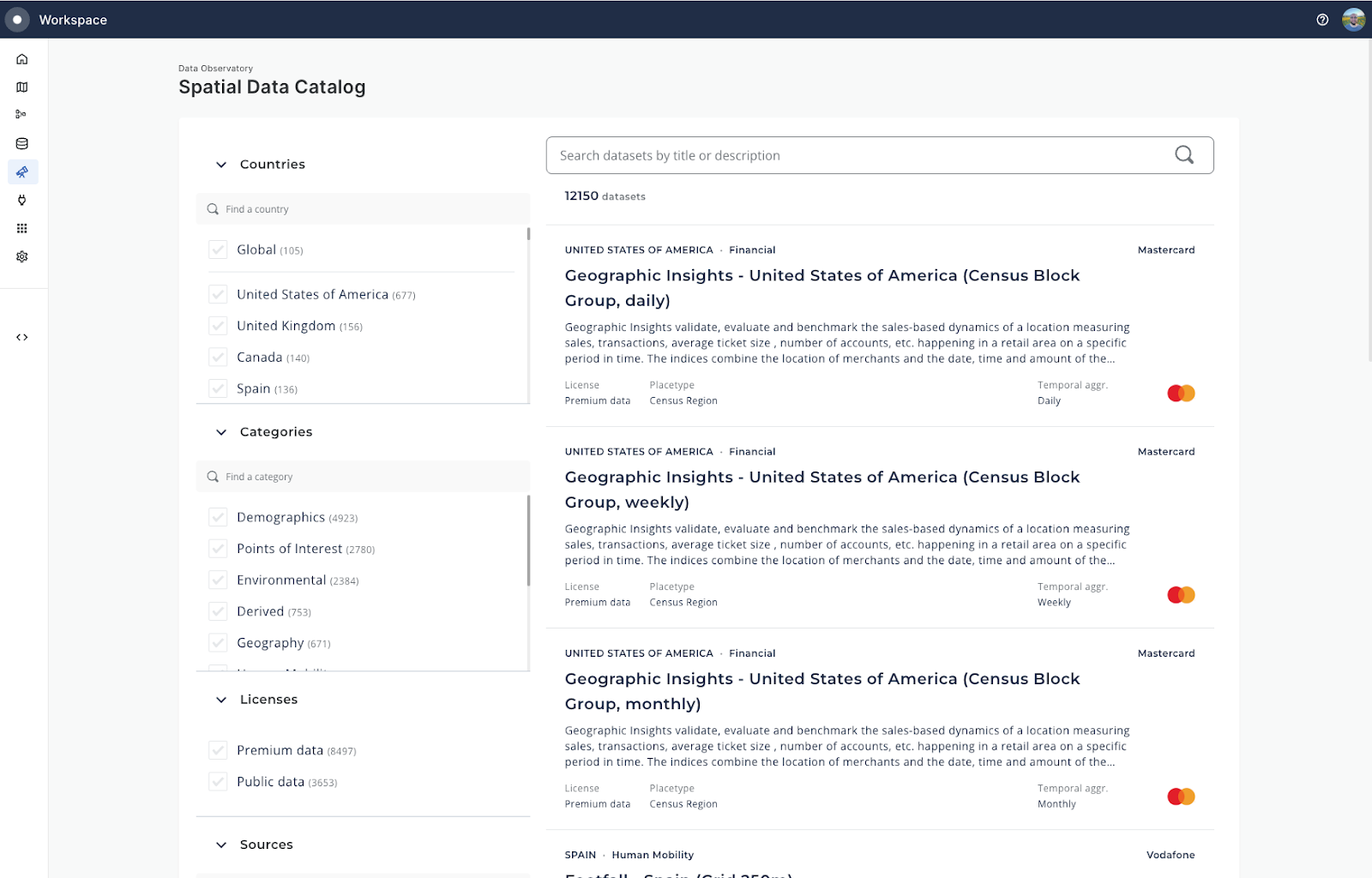
Ever heard the statistic that most people working with data spend 60-80% of their time cleaning, formatting and ETL-ing that data? We’re trying to take some of the pain out of that process with our Spatial Data Catalog. From here, you can subscribe to over 12,000 different spatial datasets from around the world, ranging from geographic boundaries to consumer spend data.
To access a dataset:
- Head to the Data Observatory tab.
- Explore! When you click on a dataset, you’ll be able to see more metadata about that dataset as well as a map and tabular preview.
- When you’ve decided you want to subscribe to a dataset, click subscribe on the preview page - and that’s it!
There are two types of subscription available: public and premium. You can access any public dataset with a CARTO account, whereas premium datasets require an additional subscription. For these datasets you will see a “Request a subscription” option and a CARTO representative will be in touch with you.
Not sure which dataset to subscribe to? We recommend subscribing to a Spatial Features dataset, which includes a range of demographic, environmental and economic data. Even better, these datasets make use of Spatial Indexes - a super lightweight type of spatial data designed for quick and efficient analysis.
Once you’ve subscribed to a dataset you’ll be taken back to the Data Explorer, but this time to the Data Observatory tab. Here you’ll see and access all of your data subscriptions and samples.
Step 4: Run some analysis
Now you know how to access your own data and subscribe to third party sources, shall we try running some analysis?
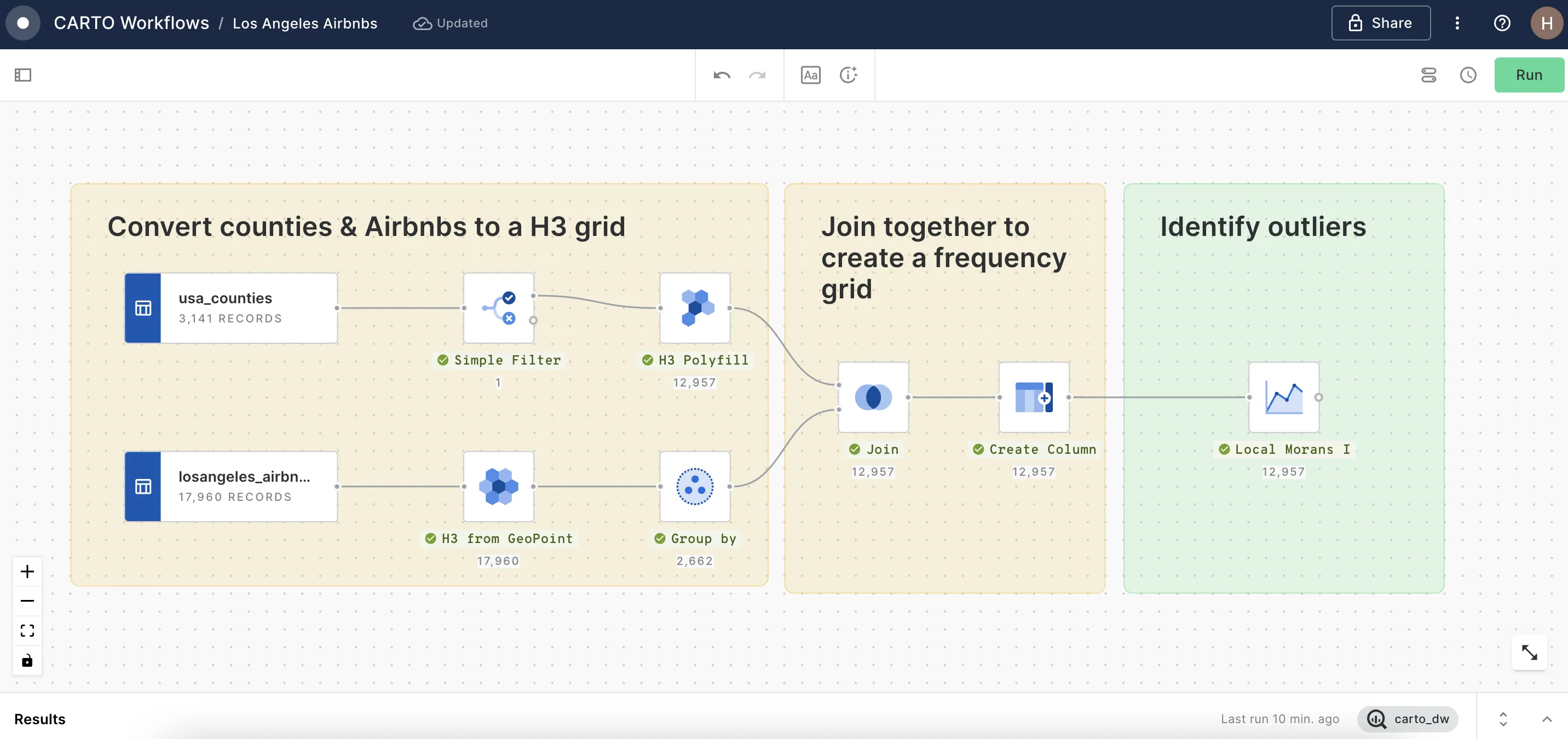
CARTO Workflows is our no-code tool for running complex spatial analysis the easy way. We have a whole range of tutorials available for you to follow in the Creating Workflows section of the CARTO Academy - you can even download pre-built Workflows templates for common spatial tasks so you don't have to build them from scratch!
An example of this in action is the workflow below, building off the Los Angeles Airbnb data we used earlier. In his workflow, the Local Morans I statistic is used to identify spatial outliers from a H3 grid of Airbnbs i.e. areas where there are few Airbnbs where you would expect many, or the reverse.
You can explore the results of this on the map below 👇
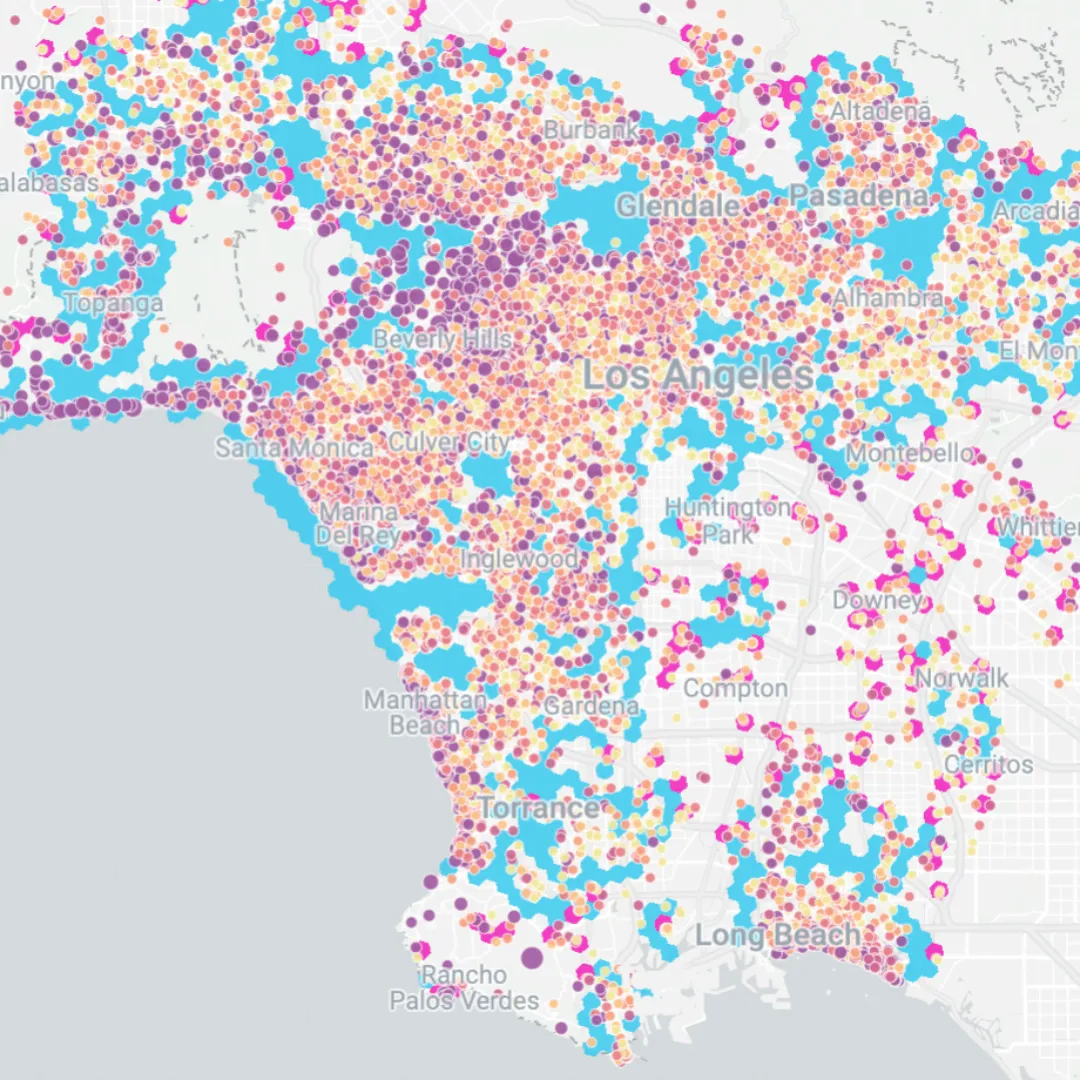
Open this map in full screen here.
Step 5: Continue learning!
So, what next?
You’ve connected to your data, created a map, subscribed to external data sources and run some simple analysis… but your Location Intelligence journey has only just started!
Head to CARTO Academy for a wide range of resources and courses designed to enhance geospatial analysis skills and empower users to leverage location data effectively. The content covers various topics, including data visualization, spatial analysis and geospatial fundamentals.
Want to learn more about how you can leverage Location Intelligence for your use case? Request a demo with one of our experts!