Raster data in BigQuery: Unlock new forms of spatial analysis
In spatial analytics, two main data types are used: raster and vector. Combining these two data formats can provide a comprehensive and powerful solution for many use-cases, more so if both types of data can be jointly analyzed in modern cloud-based data warehouse platforms such as Google BigQuery.
For those less familiar with these types of data, vector data is used to represent discrete features, such as points, lines, and polygons; with each of the geometries representing a specific feature, such as a building, a road, or a lake. Raster data, on the other hand, is often used to represent continuous surfaces, such as elevation or land cover. Raster data is made up of cells, or pixels, that are arranged in a grid. Each cell has a value that represents the attribute being measured, such as the flooding hazard at that location or the type of land cover. Learn more about the differences of these two data types here.
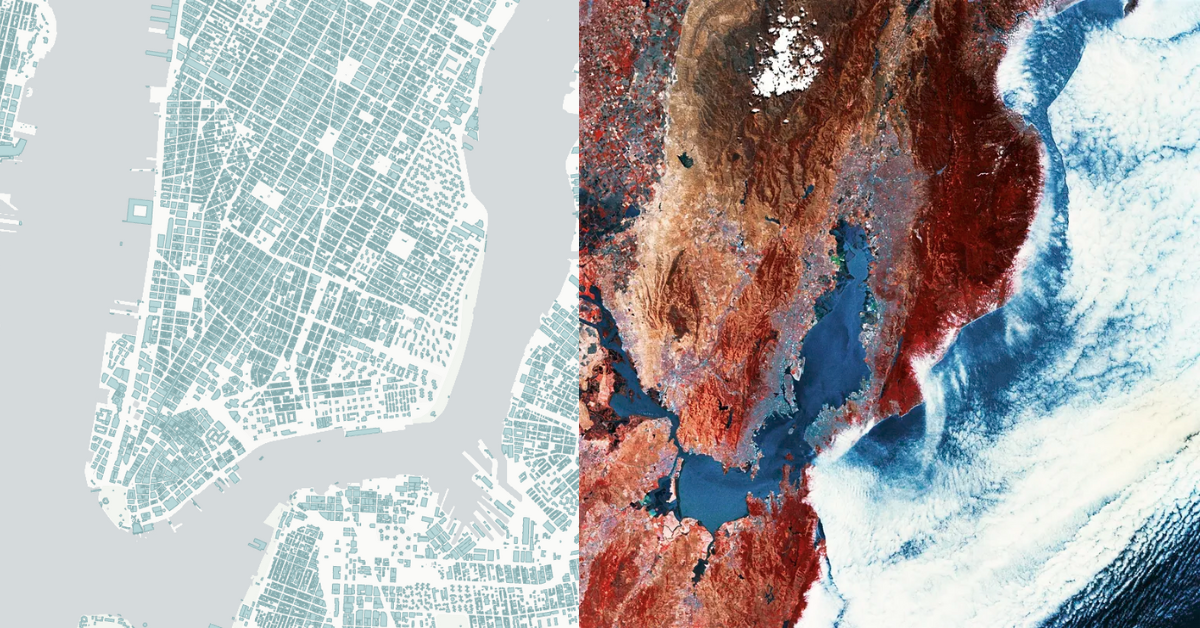
BigQuery already has a strong support for vector data with the specific GEOGRAPHY data type and many native functions to perform spatial operations, which can also be extended with our Analytics Toolbox. However, it does not have yet the support for raster data like, for example, PostGIS does.
We are happy to announce that we have recently launched in beta our raster module in the Analytics Toolbox for BigQuery, offering a set of functions to operate with raster data natively in BigQuery. These functions benefit from the processing speeds and scalability of this data warehouse.
Alongside the raster module in the Analytics Toolbox, we have also made available our Raster Loader, built in collaboration with Makepath. This publicly available Python library works as a tool for loading and optimizing GIS raster data into cloud-based data warehouses.
Why is this such a big deal?
The possibility of combining raster and vector data can provide a comprehensive and powerful solution for many geospatial analyses. Raster data, such as satellite imagery or remote sensing data, provides a detailed view of elements on the Earth’s surface (type of crops, elevation, climatology, flood models). On the other hand, vector data, such as building footprints or administrative boundaries, provide information on aspects such as topography, demographics or housing.
By overlying these two data types, one can get, for example, a complete and holistic picture of the potential impact of natural hazards and the people and infrastructure at risk from them. This in-depth analysis allows for more informed decision making in areas such as urban planning, natural resource management, real estate and insurance. Today, the computational power of cloud platforms provides the possibility to run this type of analytics at unprecedented scale and at a much more affordable cost.
To illustrate some functionality offered by the raster module, let’s work on a real example! We are going to calculate the potential risk of flooding on buildings across different areas of the south of Wales. This analysis can be useful for insurance underwriting, climate change mitigation, urban planning, real estate management etc.
In this case, we are going to analyze the average risk for flooding for buildings in the cities of Cardiff and Swansea. In order to do so we are going to use the following data sources:
- A flood hazard dataset, providing projections of fluvial, pluvial, and coastal flood inundation risks at 10 meter resolution, updated with 2020 climate state. This is raster data, kindly provided by our friends at Fathom for the south of Wales.
- A dataset with Wales building footprints in vector format, as provided by Ordnance Survey.
The goal of this analysis will be to intersect the raster and the vector datasets to obtain the risk of flooding for each building in the two cities.
Introducing CARTO’s support for raster data
We currently support raster tables that use Quadbin cells as pixels, so they require resampling the data into the Web Mercator projection used by the Quadbin spatial index.
In this example, we will reproject the raster data to a Quadbin grid in order to ensure an optimal performance. For this, we use gdalwarp and the following command:
gdalwarp -of COG -co TILING_SCHEME=GoogleMapsCompatible -co
COMPRESS=DEFLATE -co OVERVIEWS=NONE -co ADD_ALPHA=NO -co
RESAMPLING=NEAREST UKv1p1_F_rcp85_2030_10m_1in1000.tif
UKv1p1_F_rcp85_2030_10m_1in1000_Quadbin.tif
Loading raster data into BigQuery
Thanks to our new Raster Loader, available as an open source Python library, we can load our raster file into BigQuery in an effective manner. You can use it directly within the GCP console or on your local machine; to install it with pip you should run the following command:
pip install raster-loader
Now, let’s load the re-projected raster data with the flood. We can proceed to upload it to BigQuery through the carto command-line interface (CLI):
carto bigquery upload
  --file_path UKv1p1_F_rcp85_2030_10m_1in1000_Quadbin.tif
  --project <my-bigquery-project>
  --dataset <my-bigquery-dataset>
  --table UKv1p1_F_rcp85_2030_10m_1in1000_Quadbin
Storing the raster as a table in BigQuery
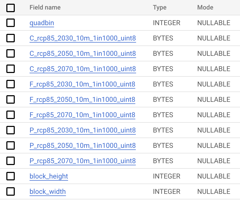
Fathom provided us with one GeoTIFF dataset for each mechanism of flooding (fluvial, pluvial, and costal), and for three year projections (2030, 2050, and 2070). The two previous steps show how to proceed with each of these files. Once all files are uploaded to BigQuery, they can be merged into a single table. In the following, we refer to this table as UKv1p1 which has the following schema:
Intersecting our vector and raster tables
Once we have our raster data in Quadbin format in BigQuery with the nine variables all in the same table, we can proceed with our geospatial analysis. In this case, we’re interested in computing the flood risk of all buildings in the cities of Cardiff and Swansea. We can easily make this calculation using RASTER_VALUE_TABLE. We only need to pass:
- the raster table containing the flood risk hazard indexes
- the vector table containing all buildings in Cardiff
- the bands and values to be extracted from the raster
- the name of the output table that will be generated with the results
The resulting table will contain one row per building with its corresponding pixel (quadbin) and bandvalues. The query below shows how this is done for the city of Cardiff. We would proceed the same way for Swansea or any other city.
CALL carto-un.carto.RASTER_VALUE_TABLE(
  ‘my-bigquery-project.my-bigquery-dataset.UKv1p1’,
  ’’’
  SELECT id, geom
  FROM my-bigquery-project.my-bigquery-dataset.cardiff_buildings
  ‘’’,
  ’’’
  C_rcp85_2030_10m_1in1000_uint8 AS coastal_flood_inundation_risks_2030,
  F_rcp85_2030_10m_1in1000_uint8 AS fluvial_flood_inundation_risks_2030,
  P_rcp85_2030_10m_1in1000_uint8 AS pluvial_flood_inundation_risks_2030
  ‘’’,
  ‘my-bigquery-project.my-bigquery-dataset.cardiff_buildings_enriched’
)
Visualizing the Quadbin rasters
Now, we’d like to visualize the building layer, together with the raster layer for fluvial flood inundation risk. Raster is stored in a compacted format in BigQuery for optimization purposes. In order to visualize this data, it first needs to be unpacked. This can be easily done with the RASTER_VALUE procedure indicating the area of interest (in our case a bounding box covering Cardiff and Swansea).
CALL
carto-un.carto.RASTER_VALUE(
    “my-bigquery-project.my-bigquery-dataset.UKv1p1”,
    ST_GEOGFROMTEXT(‘POLYGON ((-3.100891 51.436889, -3.100891 51.538221, -3.308258 51.538221, -3.308258 51.436889, -3.100891 51.436889))’),
    ‘fluvial_flood_inundation_risks_2030’,
    “my-bigquery-project.my-bigquery-dataset.UKv1p1_cardiff”
)
Open the map in full screen here.
Open the map in full screen here.
We can observe larger areas of high fluvial flood inundation risk in Cardiff than Swansea. In particular, the average risk of all buildings in Cardiff is 57.8 and 6.7 in Swansea (out of a maximum risk value of 255). This results reflects very well the fact that larger areas in Cardiff are exposed to fluvial flood inundation risk.
Also, the maps show that in Cardiff the areas at risk are a mix of residential and industrial areas, while in Swansea the area with the highest risk is an industrial area at the north of the city. This information can be very valuable for urban planning and risk exposure management in insurance.
The raster module - where will it take you?
We hope you enjoyed learning how raster and vector data types can be easily combined for extra insight! We can’t wait to see how you use this module - make sure you sign up for a two-week free trial to get started today!


