Using crime data & spatial analysis to assess home insurance risk


While the home insurance industry has historically faced challenges in adopting GIS analysis, advances in cloud-native technology are changing this. The modern geospatial tech stack makes spatial analysis faster and more accessible - enabling analysts and data scientists in the home insurance industry to generate much needed hyper-local insights at scale.
In this guide, we’ll be looking at one geospatial use case of particular interest to home insurance: crime. By understanding the crime data at individual property level, insurers can make more intelligent policy decisions - from customized pricing of premiums to tailored marketing. Read on to find out how!
Spatial Analysis of Crime Data
Crime data can be a challenging spatial dataset. It is very detailed both spatially and temporally compared to other socio-demographic data, and is also often fragmented - being reported differently by each crime authority. However, it is also an incredibly valuable dataset, allowing insurers to analyze how at risk properties are to criminal acts such as theft, arson and damage.
In the following tutorial, we’ll share how you can quickly and easily derive insights from crime data to assess insured risk. If you’d like to follow along, make sure you sign up for a free 14-day CARTO trial!
Step 1: Sourcing & Loading Crime Data
As we mentioned earlier, one of the challenges of working with crime data is that it can be very fragmented, typically being reported by local government agencies.
To demonstrate this, we’ll be basing our analysis on crime data for two adjacent locations; Los Angeles city (data available here) and Santa Monica city (data available here).
If you’re new to CARTO (welcome!) then your first step is to connect to your cloud data warehouse. For this example, we’re using Snowflake - watch the video below to see how to do this in a few simple steps.
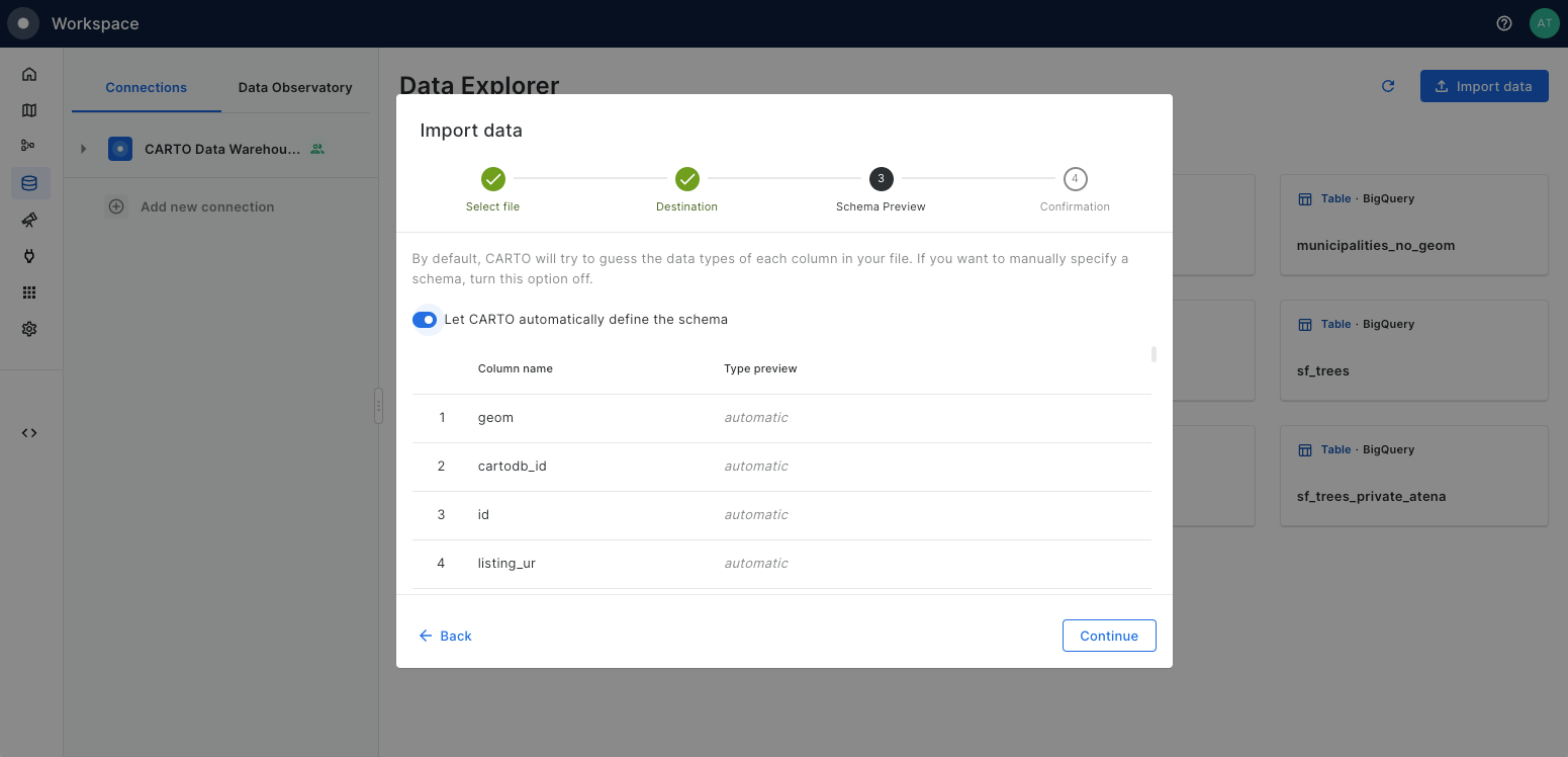
Next, you’ll need to load these tables into your Snowflake project. To do this, head to the Data Explorer tab of your CARTO Workspace and select Import data, then follow the steps to import the two tables. For this dataset we are going to deselect the Let CARTO automatically define the schema option on Schema Preview so we can manually select the correct data types for each field. In this example, you want to be sure that latitude and longitude are defined as the type float.
Step 2: Converting crime data to a H3 index
Now the data is loaded into our Snowflake project, we’ll convert the crime locations into a hexagonal Spatial Index called H3.
Spatial Indexes are a super lightweight spatial data format which are geolocated by a short reference string, rather than a geometry. In this example, we’ll explore how you can use H3 as a support geography to count the number of crimes which occur within each cell. This allows us to take advantage of its small storage requirements and lightning-fast analytical capabilities - ideal as we’re working with over 1 million input points! Find out more about Spatial Indexes in our free ebook!
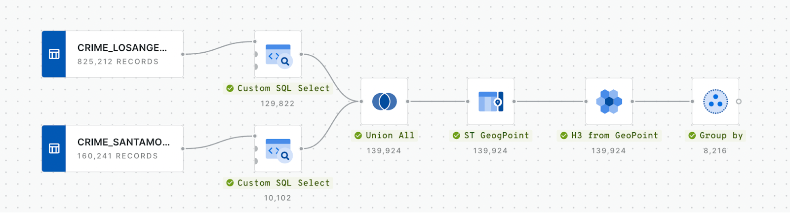
In the workflow above, we use a Custom SQL Select first to filter both input datasets so that they cover the same time period (we’ll use the last three full years - 2020, 2021 & 2022) and only crimes related to property risk (property damage, theft, arson etc). We then use Union All to merge the two tables together, and then create a point geometry for each crime (ST_GeogPoint), which is then converted to H3 cells (H3 from GeoPoint). Finally, the Group by component is used to count any overlapping H3 cells i.e. cells where more than one crime has occurred.
Let’s check out the results! Explore in full screen here.
There’s just one final piece of the puzzle we need before we can start turning our data into insights.
Step 3: Contextualizing Crime Risk
It’s not enough to just understand the number of crimes in an area; we need to contextualize it. Ten crimes occurring in a city of 1 million people doesn’t sound like much - but if those ten crimes happened in a town with 100 residents? That’s a much higher risk to properties.
To understand this, we’ll calculate the population per H3 cell using WorldPop data. This data is available free for all CARTO users for every country, at multiple resolutions and for multiple time periods. You can request a subscription directly via your Snowflake project through the Data Observatory, meaning you can keep all of your computing in the cloud.
Check out the video below to see how you can easily transform WorldPop data into a H3 index!
💡 If you’re working at the slightly coarser H3 resolution of 8, you can skip this step and subscribe to the CARTO Spatial Features dataset. This dataset - available globally - is a H3 index containing a variety of demographic, economic and environmental variables - including population!
Now we can build on our existing workflow to calculate the crime rate.
- Drag your H3 population layer onto the canvas.
- Add a Join component, inputting both the population and crime count H3 tables. Use a left join as we want to calculate the crime rate even for areas where no crimes happened.
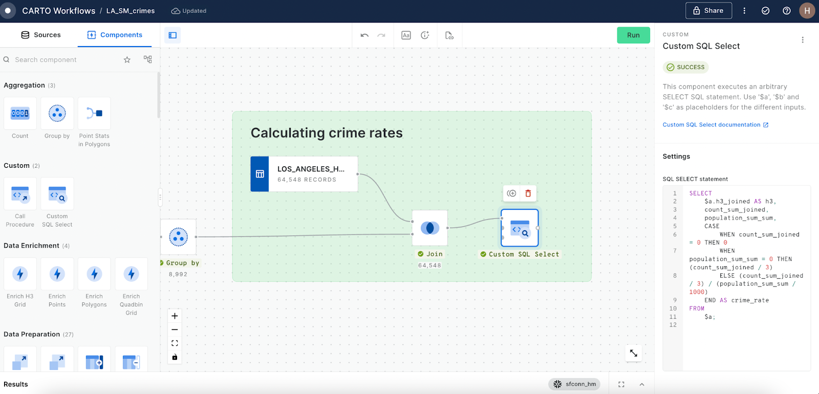
- Finally, we can calculate the crime rate! Normally you would just add a Create Column component to do this, but as we have some zeros and nulls in our data, we need to do an additional calculation using the Custom SQL Select component. Use the below SQL to calculate the number of crimes per year (of the 3 sample years) per 1,000 residents. Note how we can use the placeholder $a to call the attached component.
SELECT
    $a.h3_parent AS h3,
    count_sum_joined,
    population_sum_sum,
    CASE
        WHEN count_sum_joined = 0 THEN 0
        WHEN population_sum_sum = 0 THEN (count_sum_joined / 3)
        ELSE (count_sum_joined / 3) / (population_sum_sum / 1000)
    END AS crime_rate
FROM
    $a;
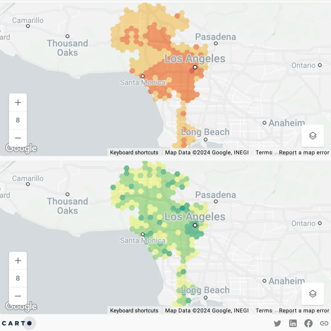
Let’s check out the crime rate in comparison with the crime count! Open in full screen here.
Step 4: Property-level crime statistics
While it’s helpful to understand crime rates on a city level, insurers need to be able to pinpoint what’s happening at the individual property level - so let’s do that!
Using Los Angeles County Property Parcels as our source (which includes a helpful field on the price of each property when last sold), we can add a final section onto the end of our workflow where we:
- Use a H3 from GeoPoint component to convert each property to a H3 index (remember to set this as resolution 9; the same as all of our other H3 layers).
- Join the crime rate data to the property H3 layer by the H3 columns in both tables.
Check the whole workflow out in action below!
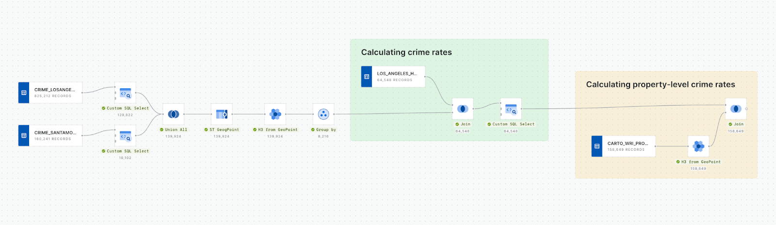
Now we have a crime rate for each property! By converting our two input datasets - crime rate and properties - to H3 indexes, we are effectively replacing a heavy and slow spatial join operation with a fast and effective string-based join. The results? Crime rates for 159 THOUSAND properties in seconds!
Shall we see what that looks like?
Step 5: Data-driven decision making
Check out the results of our analysis on this map!
With property-level crime rates in hand, home insurers can now make more informed decisions, including;
- Geosegmentation & customized premium pricing: Categorizing areas by crime risk for tailored coverage and setting premium pricing levels based on inferred risk.
- Risk Mitigation: Offer advice and incentives for home security improvements.
- Targeted Marketing: Focus awareness campaigns on homeowners in specific risk areas.
- Fraud Detection: Use crime incidence data to identify suspicious claims patterns.
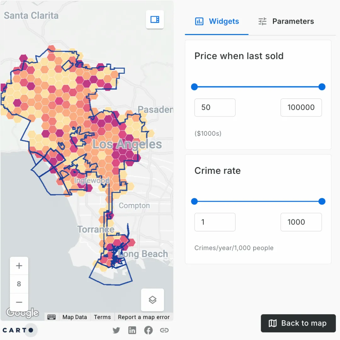
💡We’ve added some features to help users navigate our analysis, including zoom-defined rendering to ensure the detail at different zoom levels is appropriate and SQL parameters to allow end-users to filter the data to the geographic area of interest.
❄️🗺️📈
Ready to start scaling your decision making with cloud-native geospatial analysis? Sign up for a free 14-day CARTO trial today!