Using trade area analysis for CPG merchant segmentation


Understanding customers (commonly referred to as “merchants” within CPG) and prioritizing which are the best points of sale to place products is as important now as ever for brands. According to McKinsey despite the rapid growth of e-commerce traditional distribution channels still represent the largest share of sales in the consumer market. Furthermore in developing markets CPG companies are expanding their physical customer networks making insights relating to expansion planning crucial for success.
Another challenge is where to spend trade promotion budget given it is an important cost component directly affecting their margins. While trade promotion performance measurement and optimization is the most important step to be taken for CPG transformation (according to Google Cloud) using data-driven approaches to better understand customers can help inform and optimize trade promotion decisions.
For many CPG companies these activities are an even greater challenge due to the lack of up-to-date and granular customer sales data for their product portfolios. In the absence of this data constructed proxies using geospatial insights can help them define consolidated channel strategies for their complex networks of merchants.
Announcing our new CPG module in the Analytics Toolbox for BigQuery
In this blogpost we will showcase how CPG data scientists and analysts can now leverage CARTO’s Analytics Toolbox for BigQuery to segment their customers or merchants based on the characteristics of their trade areas.
The Analytics Toolbox provides a complete framework of analysis capabilities to perform spatial analytics in SQL computed natively in the leading cloud data warehouse platforms. Our implementation for BigQuery enables a fully cloud native spatial analytics and Spatial Data Science experience whilst reaping the benefits around privacy compliance scalability and the lower costs that cloud data warehouse infrastructure brings.
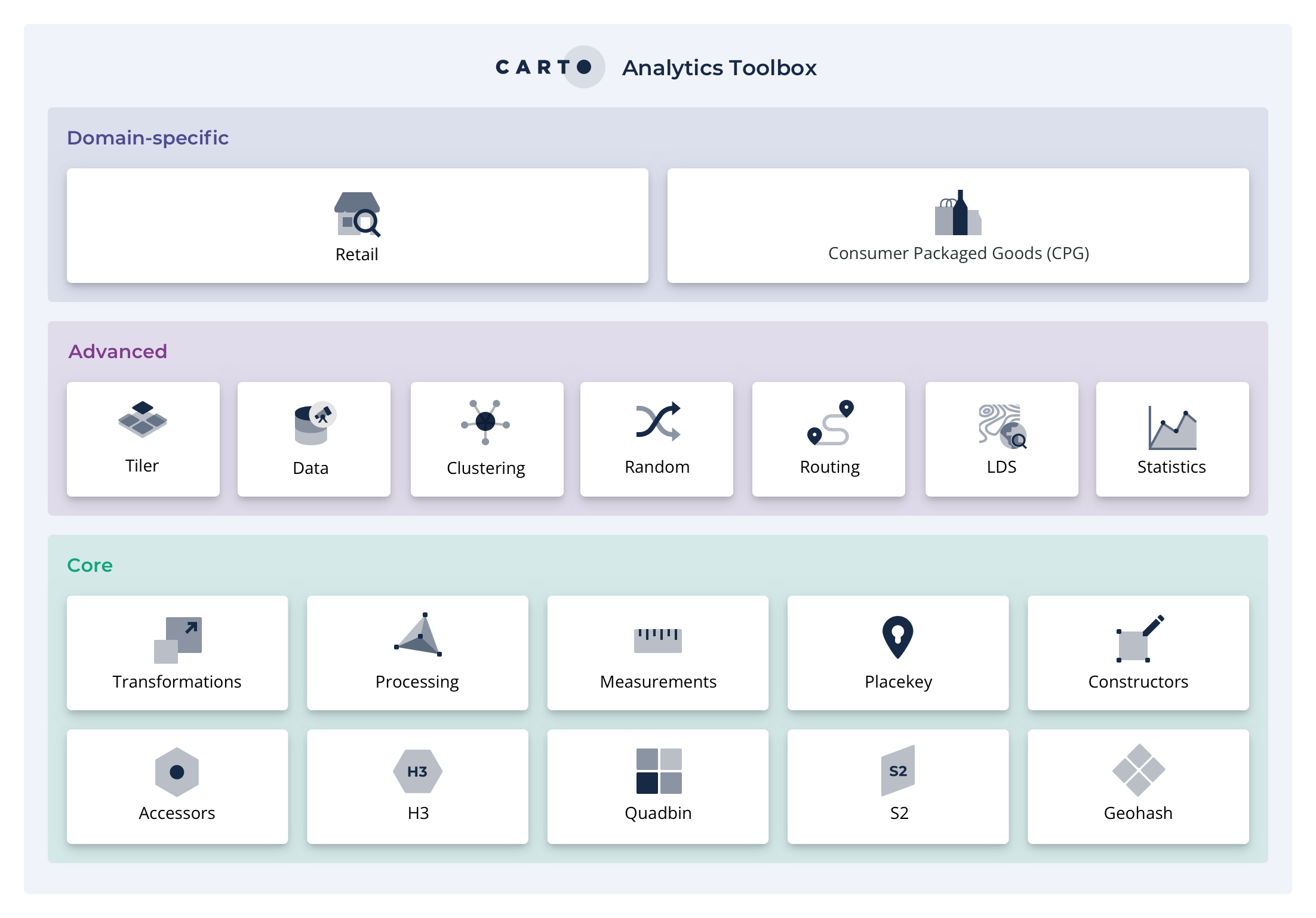
The analysis routines in the Analytics Toolbox cover a broad range of spatial analytics use cases and are organized into a series of modules (data clustering statistics etc.) based on the functionality that they offer. Today we are happy to announce the availability of a new domain-specific module to solve geospatial analytics for the CPG / FMCG sector starting with Customer Segmentation.
Segment your customers
In order to unlock customer segmentation analysis we have implemented three new procedures into the Analytics Toolbox that cover all the necessary steps to solve this use case end-to-end: trade area generation data preparation and customer segmentation.
- GENERATE_TRADE_AREAS: This procedure allows the user to create trade areas based on different strategies around a set of customer / merchant locations. Users can select the type of trade area to be defined (among buffer kring isoline) and provide the associated parameters (for example for a buffer the parameter is distance). The method returns a table of customer IDs and locations and associated polygons for the trade area (including the type of trade area and configuration).
- CUSTOMER_SEGMENTATION_ANALYSIS_DATA: This procedure prepares the data to be used in the customer segmentation analysis. It takes as an input the trade area of each customer (merchant location and its associated trade area) along with already incorporated features and it enriches it with additional features selected by the user from external datasets. These features can either be from the user’s own proprietary data or from third-party data from CARTO’s Data Observatory subscriptions. This method leverages the DATAOBS_ENRICH_POINTS DATAOBS_ENRICH_POLYGONS and ENRICH_POLYGONS methods available in the data module of the Analytics Toolbox.
- RUN_CUSTOMER_SEGMENTATION: This procedure takes as an input the output of the previous method or any adapted form of it and performs clustering (using the K-means method) based on the user's defined number of output segments (it can be a single number of output segments or multiple should the user want to run multiple segmentation scenarios). In addition the capability of performing dimensionality reduction before clustering is offered in order to limit the impact of multicollinearity to the clustering. The output gives the customers´ locations assigned to segments as well as a series of descriptive statistics that focus on features (e.g. the percentiles of the entire input data and of each segment for each variable) or that focus on the quality of the model output (e.g. Davies-Bouldin index mean squared distance).
Identifying the best restaurants and cafes in the Bay Area to promote a new healthy premium beverage
In this example we will segment restaurants and cafés in the Bay Area (San Francisco Marin San Mateo Contra Costa Alameda Santa Clara) to identify optimal areas to promote a hypothetical healthy premium beverage for younger audiences.
In terms of data we assume that we as the CPG company own a dataset with the location of our merchants plus competitor merchants within our network. For this data we have leveraged SafeGraph’s Places dataset. We will then enrich the trade areas of these merchants with AGS Sociodemographics and Consumer Spending data Spatial.ai Geosocial Segments and PersonaLive datasets human mobility data from Unacast Activity and again SafeGraph’s Places data for Point of Interest. All these sources come from the premium data offering in CARTO’s Data Observatory.
Trade Area definition
First we filtered the Safegraph Places data to keep only restaurants and cafeterias in the area of interest. Then we defined the trade area for each location based on their urbanity level which we extracted from the CARTO Spatial Features dataset. For an area in California where distances are much more commonly covered through private transportation methods we used larger trade areas for medium and low urbanity locations. Specifically:
- For “high urban density” & “very high urban density”: A buffer of 500m radius.
- For “medium urban density”: A buffer of 5km.
- For “remote” “rural” and “low urban density”: A buffer of 15km.
Find below a sample code snippet which creates trade areas of 15km buffers for restaurant locations in remote rural and low density urban areas in a selected area in California. The customer query is custom and selects the locations for which we would like to create trade areas. The rest of the query represents the characteristics of the trade areas to be generated.
CALL `carto-un`.carto.GENERATE_TRADE_AREAS(
   --customer_query; identifying restaurant merchants in rural locations in California
    '''
    SELECT a.geoid as store_id   geom
    FROM `<my-project>.<my-dataset>.merchants` a
    JOIN `<my-project>.<my-dataset>.sub_carto_derived_spatialfeatures_usa_h3res8_v1_yearly_v2` b on `carto-un`.carto.H3_FROMGEOGPOINT(geom 8)=b.geoid
    JOIN `<my-project>.<my-dataset>.california_buffer` on ST_INTERSECTS(geom buffer_geom)
    where closed_on is NULL and b.urbanity in ('remote' 'rural' 'Low_density_urban')
    AND CONTAINS_SUBSTR(top_category 'Restaurants and Other Eating Places')
'''
    --selecting the method
    'buffer'
    --method options
    "{'buffer':15000.0}"
    --output_prefix
    '<my-project>.<my-dataset>.low_urban'
-- This is sample code  not aimed for reproducing the analysis
)
A user can run this method once for each level of urbanity and join the output tables. For example in our case they would have to run the method three times to create buffers of 500m 5km and 15km radius for merchants located in areas characterized by a different level of urbanity.
Note that beyond ‘buffer’ there’s also the option to generate the trade areas based on drive or walk time isolines.
Data enrichment
The next step is to enrich these trade areas with relevant features. These features should help us understand where our product has a higher chance of being successful. They can also identify subtle differences between customer segments to adapt business development and trade promotion strategies.
In our case we consider the following features would be the most relevant in this exercise:
- Sociodemographics:
- Total population, Median age, Median income 18-24, Median income 25-34, Median household income;
- Consumer spending:
- Food and beverage expenditure (at home and out of home);
- Human Mobility:
- Aggregated number of visitors per area observed for the months of January, April, July and October;
- Points of Interest:
- Total number of restaurants and cafés in area;
- Household behavioral segments:
- Ultra-wealthy, Wealthy-suburban, Upper suburban, Educated urban, Young professionals, Young Urban, Rural High income, Rural average income.
- Geosocial behavioral segments:
- Hipster culture, Trendy eaters, Ingredient attentive, Fueling for Fitness and Fitness Obsession.
In the sample code snippet below we enrich a table with trade areas with sociodemographic and consumer spending variables from the Data Observatory.
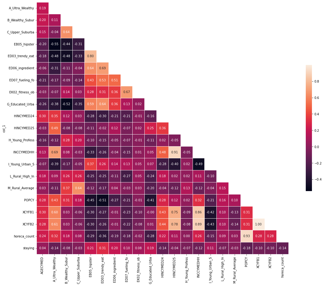
The output of this method is a table of enriched trade areas a table with correlation values between variables and a table of descriptive values for each variable (mean median standard deviation etc.)
CALL `carto-un`.carto.CUSTOMER_SEGMENTATION_ANALYSIS_DATA(
-- Select the trade areas of merchants  can be pre-enriched trade areas
  R'''
  SELECT *
  FROM `<my-project>.<my-dataset>.trade_areas_enirched`
  '''
  -- Data Observatory enrichment - Only for sociodemographics and consumer spending categories
    [("POPCY_6657e7c4"  'sum')  ("AGECYMED_d9cf8a34" 'avg') ("INCCYMEDHH_ce22a17e" 'avg') ("HINCYMED24_52e71e33" 'avg') ("HINCYMED25_25e02ea5" 'avg') ("XCYFB1_34f3df35" 'avg') ("XCYFB2_adfa8e8f" 'avg')]
  '<my-dataobs-project>.<my-dataobs-dataset>'
   – Custom data enrichment
   NULL  NULL
 –output_prefix
   ‘<my-project>.<my-dataset>.california_test’
– This is sample code  not aimed for reproducing the analysis
)
After the enrichment we used the correlation analysis table to understand the relationship between all pairs of features. In the diagram below we can see that very few features are correlated with each other. The one relationship that stands out the most is the relationship between average median income and the household expenditure in food away/home. In addition the total population correlates with the number of HORECA (Hotels Restaurants Cafeterias) stores. From a business perspective these relationships make sense the higher a household income is the more it can spend on food; while for the second more densely populated areas are likely to have more restaurants cafeterias etc.
Customer segmentation
Finally we run the segmentation function using a combination of target segments in this case 4 5 6 7 and 8 segments.
Below a sample code snippet where we segment the enriched trade areas table an output from the CUSTOMER_SEGMENTATION_ANALYSIS_DATA method. We ask the method to segment 5 times. The first time it will divide trade areas into 4 segments the second time into 5 segments and so on.
CALL carto-un.carto.RUN_CUSTOMER_SEGMENTATION(
–select the source table of merchants enriched with geospatial characteristics
  ‘<my-project>.<my-dataset>.california_test_enrich’
–select the number of clusters to be identified (five analyses to identify 4  5  6  7 and 8 clusters respectively)
   [4  5  6  7  8]
–PCA explainability ratio
   0.9
–output prefix
   ‘<my-project>.<my-dataset>.california_test_clustering’
);
The main output of this method is a table assigning each merchant to a segment for each combination of target segments. In addition a table with the descriptives of each variable for each analysis a table with the statistics of the analysis (Davies-Bouldin index Mean-squared distance) and a table with the results of the PCA analysis.
The Davies-Bouldwin index and the mean squared distance for all the combinations are shown in the table below.
| num_clusters | davies_bouldin_index | mean_squared_distance |
|---|---|---|
| 4 | 1.25 | 13.72 |
| 5 | 1.90 | 12.07 |
| 6 | 1.62 | 10.45 |
| 7 | 1.61 | 9.81 |
| 8 | 1.61 | 9.89 |
Exploring the resulting segments for each scenario (i.e. for different numbers of clusters) we identified the combination of 7 segments to be the best performing for our given geography selected POIs trade area configuration and selected features. The assessment consists of an objective criteria (Davies-Bouldwin index and the mean squared distance) along with the subjective criteria business logic and interpretation of the outcomes. The best theoretical separation amongst clusters is for the case of 4 clusters. However inspecting the results along with the similarities of stores within clusters the case of 7 clusters is deemed as the most appropriate one.
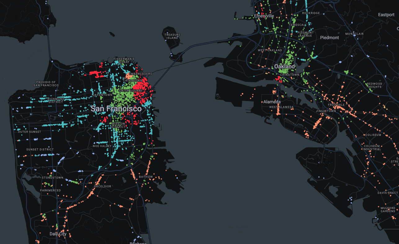
See the map below for the results:
Let’s take a closer look at the characteristics of each resulting segment.
| ID | Segment name | Number of merchants | Description |
|---|---|---|---|
| 1 | Low population density urban | 2.5k | Characterized by a lower population density (mostly for a 500m radius) yet higher income for younger population and higher spending on food and beverage; higher presence of the Educated Urban consumer segment. |
| 2 | Rural higher income lifestyle | 1.8k | Characterized by high residential density for rural trade areas high income individuals. It is also characterized by a higher presence of the Young Professionals segment. |
| 3 | Focus on essentials | 4.1k | Characterized by lower income per household also for younger ages. The segment experiences a lower density of merchants. Presence of relevant consumer segments is also lower. |
| 4 | Rural higher income lifestyle | 0.3k | Similar to segment 4 also characterized by a higher presence of the Ingredient Attentive and Fitness Obsession segments. |
| 5 | Health conscious and spending conscious | 4.5k | Characterized by high presence of all relevant consumer segments high mobility. Income is lower also for younger age groups; by effect spending on food and beverage is lower. |
| 6 | Tech sector areas | 6.1k | High presence of Ultra-wealthy individuals higher median income for younger population and higher spend on food both outside and inside the household. |
| 7 | Health conscious and premium lifestyle | 1.2k | Similar characteristics to segment 5 however in this segment income and as a consequence food and beverage spend are much higher. |
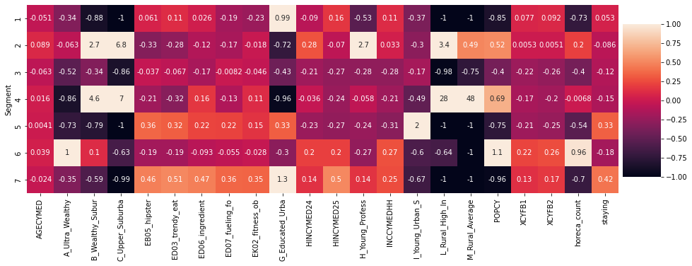
You can see in the heatmap below the characteristics of each segment in a more visual format. A cell represents the value of the feature (horizontal axis) for a Segment (vertical axis). This value is the percentage difference between the average value for that segment and the global average value.
Conclusions
In this study we have explored the Bay Area to understand where and how we could promote a new healthy beverage. We used clustering techniques to divide restaurants and cafeterias into discrete segments based on their trade area characteristics.
We have identified and named 7 segments based on the trade area characteristics for target merchants.
Even though there is a potential strategy for all identified segments we would prioritize segments 1 (Low population density urban) 5 (Health conscious and spending conscious) and 7 (Health conscious and premium lifestyle). The decision is based on a combination of interest in healthy ingredients and fitness adequate income and higher spending on food and beverage.
To launch the product we would focus on a segment with high income potential and lower cost to distribute. This could be Segment 7 (i.e. “Health conscious and premium lifestyle”) based on the higher affinity to health and fitness interests higher spend on food and beverage and smaller segment size.
Having understood the segments we would then identify high potential hotspots within. To do that we can run further analysis to identify smaller areas of higher relevant interest or higher food and beverage spend for example using techniques such as spatial indexing.
The customer segmentation procedures are now available from the Analytics Toolbox for BigQuery and can be run directly from the BigQuery console or from your SQL or Python Notebooks using the Python client for BigQuery.
Want to try it for yourself? Sign up for a free 14-day trial of the CARTO platform today!