How To Optimize Location Planning For Wind Turbines
With a global goal of reaching net zero by 2050, renewable energy sources such as solar energy, wind power, and other forms of kinetic energy, are set to play a huge role in powering us through the 21st century and beyond. It is estimated that an additional 70-80 GW of wind power that creates electricity will need to be installed annually to reach net zero.
While the future for wind power looks bright, one of the biggest questions facing organizations looking to drive this growth from renewable energy projects is… where?

Site Selection for wind farms represents a challenging contradiction for spatial analysts. The ideal location should be somewhere remote but not too remote. Not too close to residents, but with a sufficient power and transport infrastructure able to support construction and operations. A site should experience high wind speeds (often found in upland areas) but should not be ecologically sensitive to avoid the energy development causing negative environmental impacts.
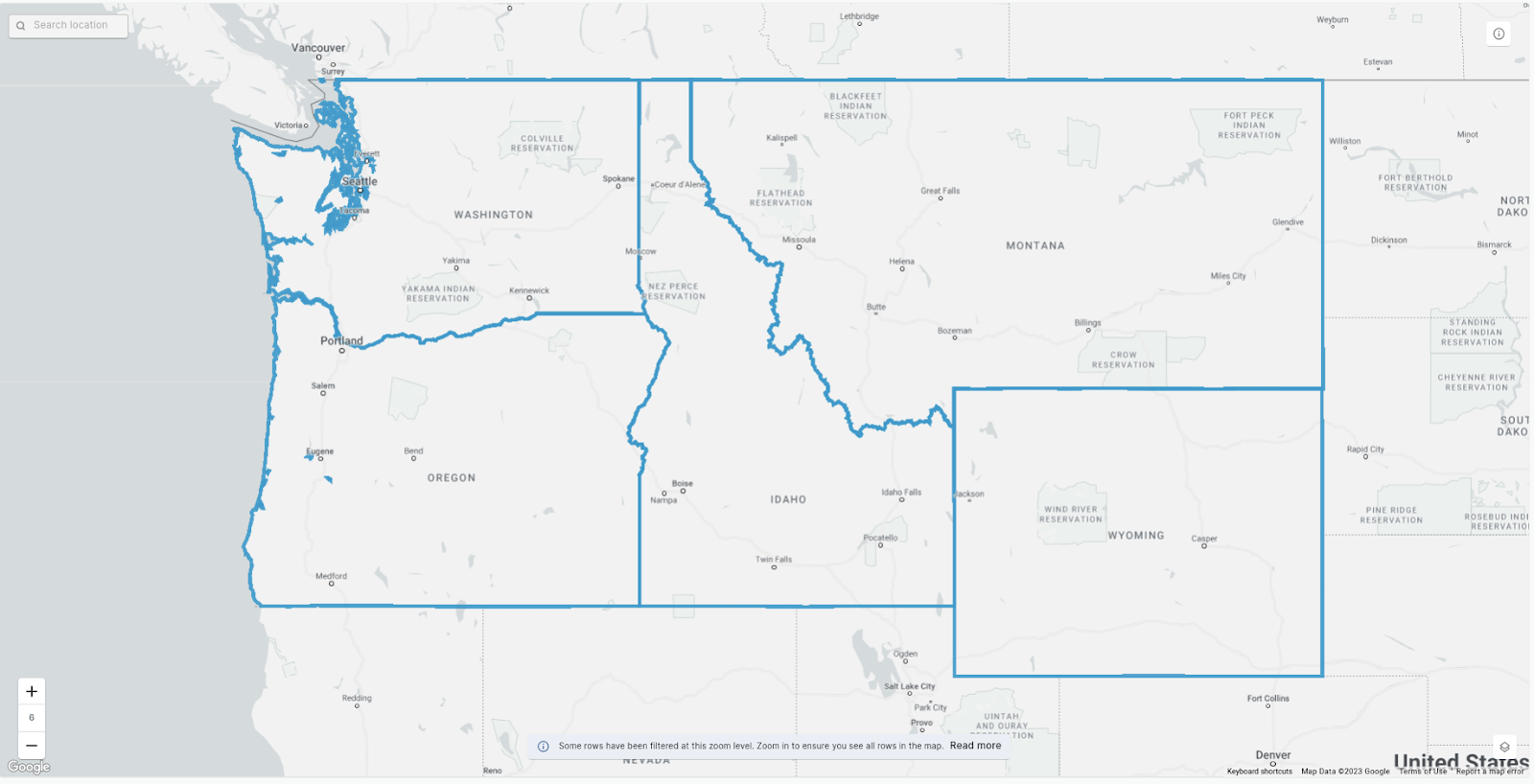
In this guide, we’ll be seeking sites in the north west of the USA which meet these contradictory criteria. Make sure you grab a free two-week CARTO trial here so you can try out this analysis yourself!
Multi-criteria analysis for wind turbine Site Selection
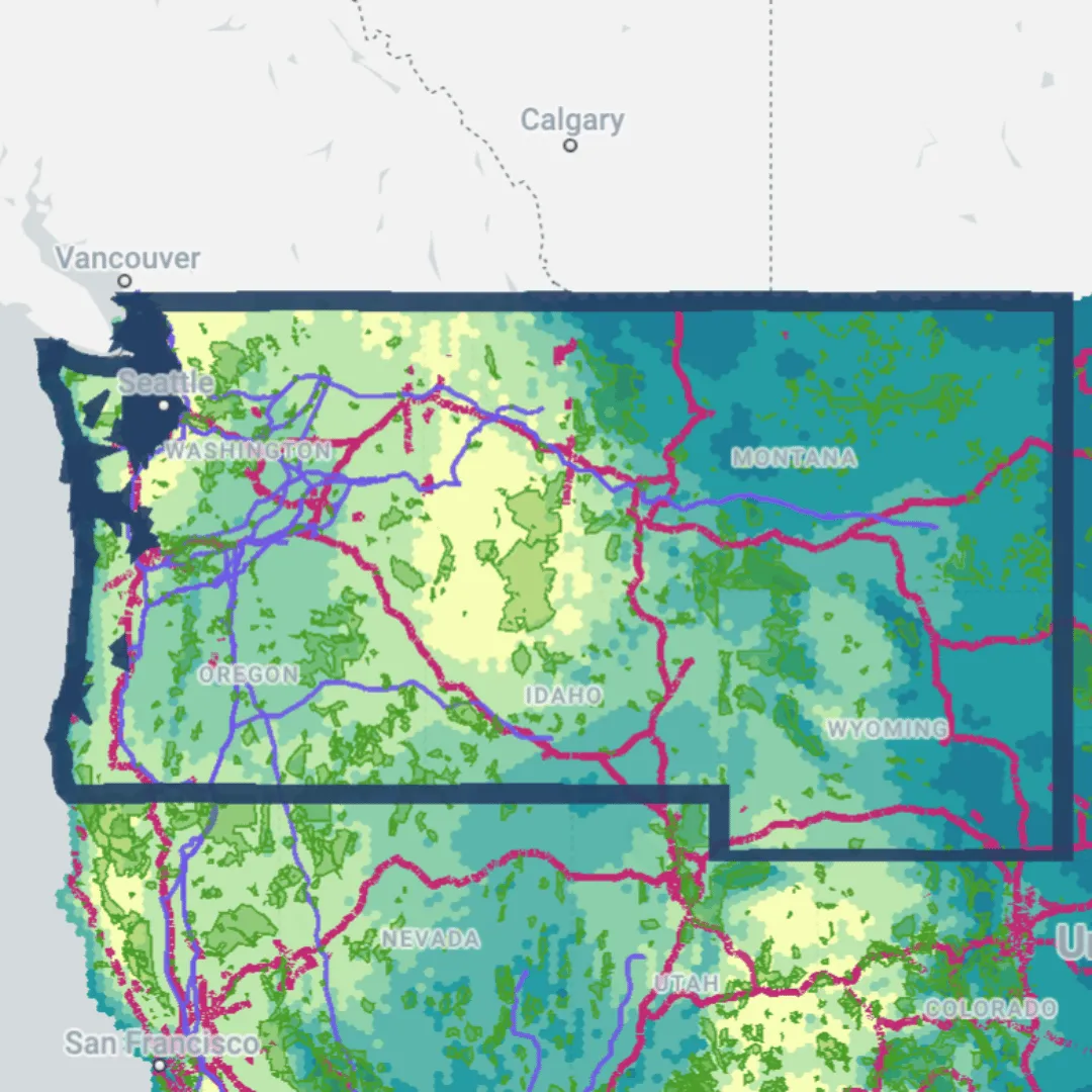
For our Site Selection process, we’ll have two criteria types; boolean and ranked. Boolean criteria will return a yes or no based on specified conditions; locations will be discarded if they don’t meet these. Ranked criteria will be used to rank the remaining locations in terms of suitability.
Please note that this guide is intended as an illustrative guide to the types of data and analysis which can be used to optimize the potential locations of wind farms; it is not intended to be exhaustive of all considerations.
Boolean criteria
- Must be within 25 miles of a >=400KV powerline, with data sourced from the Homeland Infrastructure Foundation.
- Must be within 15 miles of a motorway or trunk level highway.
- Must not intersect a large protected area (please note Native American lands are not included as many Native American communities are reported to be pro wind farm developments).
The highway and protected area (see definition here) data were sourced from OpenStreetMap - a fantastic global free database often dubbed “Wikipedia for maps.” While the crowdsourced nature of this dataset means quality and consistency can vary, major highways and protected areas are typically accurate due to their significance.
You can access this data for free from the Google BigQuery OpenStreetMap public dataset by modifying the below code. This code extracts protected areas which intersect our selected states (accessible via our Spatial Data Catalog here). Note you’ll need to change “xxxxxxxx” to your Data Observatory dataset - you can find this in the sample SQL code for any dataset you have a subscription to. This code also extracts only areas which have an area greater than or equal to 0.73km². Why? This is the average area of a H3 cell at resolution 8, which is the geographic support system we’ll be using for this analysis (keep reading for more information).
You can read our full guide to working with the BigQuery OpenStreetMap dataset here.
WITH
 aoi AS ( SELECT ST_UNION_AGG(geom) AS geom
 FROM `carto-data.ac_xxxxxxxx.sub_carto_geography_usa_state_2019`
 WHERE do_label IN ('Washington', 'Oregon', 'Idaho', 'Montana',  'Wyoming')),
protected AS (
SELECT
  (SELECT osm_id) osmid,
  (SELECT value FROM UNNEST(all_tags) WHERE KEY = “boundary”) AS boundary,
  (SELECT value FROM UNNEST(all_tags) WHERE KEY = “name”) AS name,
  (SELECT geometry) AS geom
FROM bigquery-public-data.geo_openstreetmap.planet_features)
SELECT protected.*
FROM protected, aoi
WHERE ST_CONTAINS(aoi.geom, protected.geom) AND protected.boundary = ‘protected_area’) AND ST_AREA(protected.geom) >= 737327.598
Ranked critera
Following this assessment, locations will be ranked based on the following criteria:
- Average wind speeds, with higher speed being preferable
- Lowest population within 18.6 miles or 30 kilometers; the distance beyond which visual impacts from wind farms are deemed negligible.
This data will be extracted from our Spatial Features dataset, available via our Spatial Data Catalog here. These tables include data on demographics and climatology. In this instance, we’re interested in the total population and average monthly wind speed.
We’ll be using the H3 version of this dataset. H3 is a Spatial Index; a global, multi-resolution grid system which is geolocated by a short reference ID rather than a long geometry string. This makes Spatial Indexes small to store and super quick to analyze - ideal for large-scale yet detailed analyses like this!
Want to know more Spatial Indexes? We’ve written a whole ebook about them which you can download for FREE here!
Explore these input variables for the whole of the US in the map below!
A low-code analytical framework
For this analysis, we’ll be using CARTO Workflows - a visual, low-code analytics tool currently in beta.
Boolean criteria
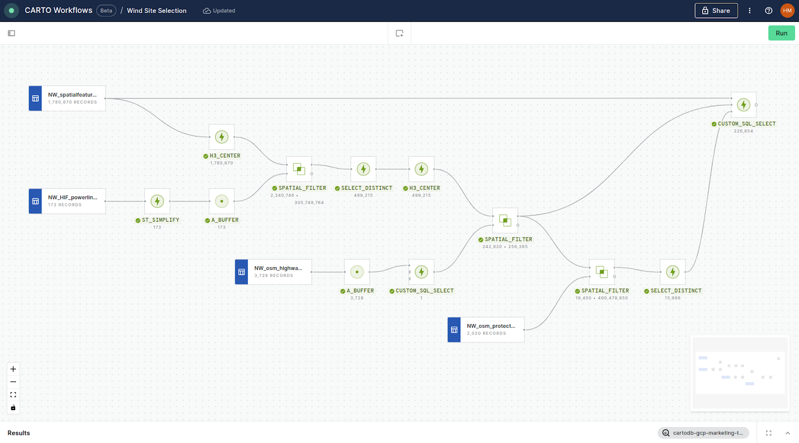
This workflow filters our Spatial Features H3 dataset from the 1,780,870 cells which cover our study area, down to the 226,854 features which meet our criteria. Let’s break this down to see how it works!
Step 1: Select cells within 25 miles of a >=400KV powerline
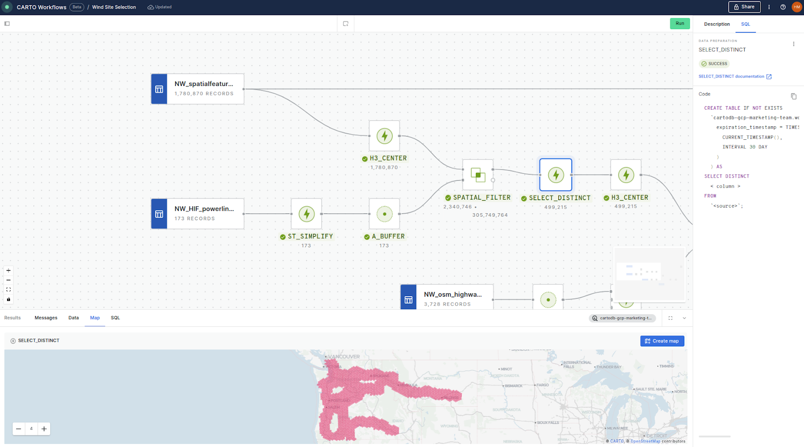
In this first section of the analysis we:
- Convert the H3 table “NW_spatialfeatures” to their center points using H3_CENTER, as a geometry field is required for the subsequent step.
- Simplifies the geometry of “MW_HF_powerlines” using ST_SIMPLIFY to improve the processing speed of the subsequent steps. A_BUFFER is then used to create a buffer of 25 miles around the powerlines.
- A SPATIAL_FILTER component is then used to select only H3 centroids which intersect the buffers. If you want to learn more about Spatial Filters, check out this guide.
- As the buffer layer contains multiple geometries, it is likely that some H3 cells intersect with more than one buffer which would generate duplicate cells during the filter. Therefore, the final step of this section is to use SELECT_DISTINCT to eliminate duplicates.
The 499,215 resulting cells can be seen in the map preview at the bottom of the Workflows screen.
Step 2: Select cells within 15 miles of a major highway
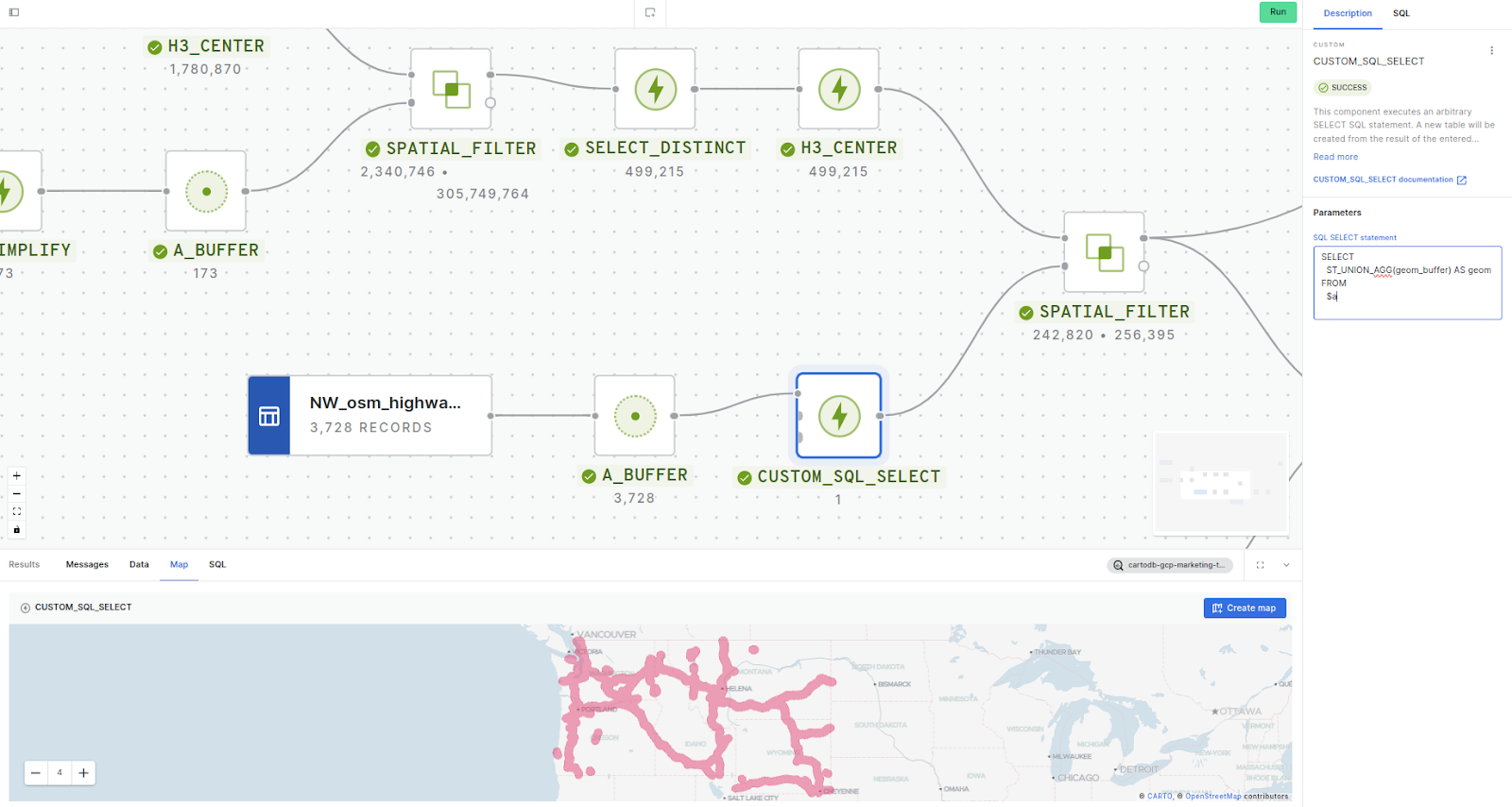
- As with the previous section, first we need to use H3_CENTER to create centerpoint geometries from our H3 table, this time using the results of step 1.
- We then repeat the steps from section 1, this time using the table “NW_osm_highways” and a buffer distance of 15 miles. However, as our highway table contains 3,728 unique geometries, there is the potential for the creation of a lot of H3 duplicates during our Spatial Filter, which could slow things down significantly. To combat this, we’ve added a CUSTOM_SQL_SELECT and used the ST_UNION_AGG function on the results of A_BUFFER to merge all of the buffers into one feature. Note how we can use $a to call the first connected inputs (or $b and $c if multiple inputs are connected).
SELECT
ST_UNION_AGG(geom_buffer) AS geom
FROM
$a
- And finally run another SPATIAL_FILTER to select only the H3 cells which intersect the buffer, taking us down to 242,830 cells - we're getting there!
Step 3: Deselect cells which intersect a large protected area
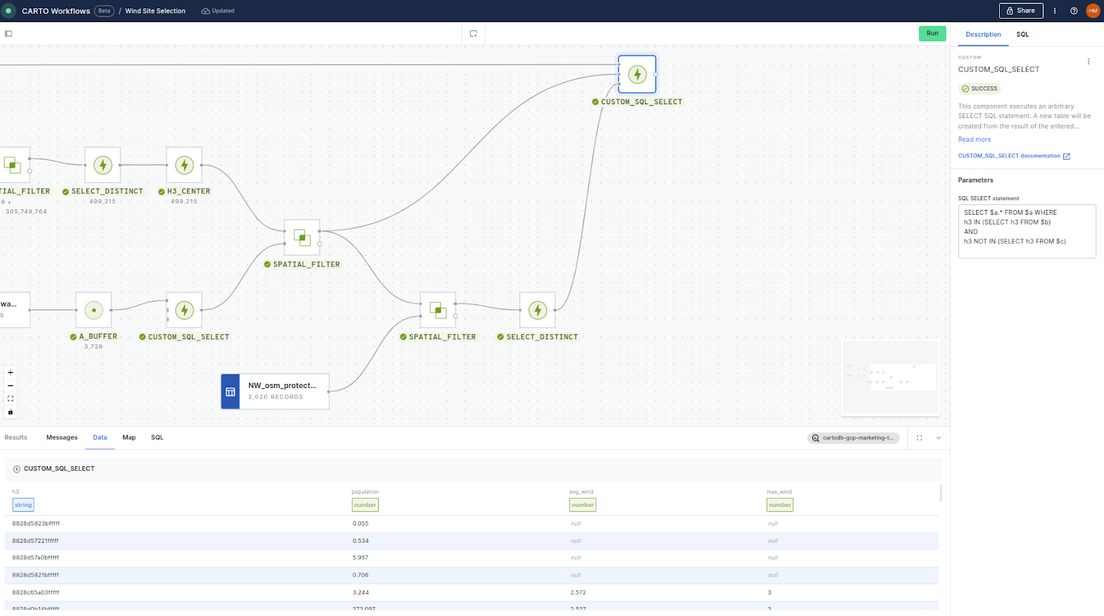
Nearly there! This final section is a little different.
- We run another SPATIAL_FILTER; this time we use this to establish which H3 cell centers intersect the protected areas.
- Again, H3 cells could potentially intersect multiple protected areas which would create duplicates, so we’ll use SELECT_DISTINCT to remove these.
- And finally, we want to select the H3 cells from our original table (which contains the population and wind variables needed for the second half of our analysis) which intersect with the powerline and highway buffers, but do not intersect with the protected areas.
To do this, we connect the original table, the resulting SPATIAL_FILTER from step 2, and the resulting SELECT_DISTINCT from step 3 to another CUSTOM_SQL_SELECT component. We then use the following SQL code to select the required H3 cells:
SELECT $a.* FROM $a WHERE
h3 IN (SELECT h3 FROM $b)
AND
h3 NOT IN (SELECT h3 FROM $c)
Finally, add a SAVE_AS_TABLE component to the end of this - and let’s take a look at what we’ve got!
Ranked criteria
Now we have our potential locations for a wind farm, we can rank their suitability. We already have the average wind speeds, but we still need to calculate the population size within 18.6 miles / 30 kilometers of each cell.
Step 4: Calculating population within a distance
Using traditional geometries, this would be a really expensive and slow operation. Thankfully, Spatial Indexes make this much faster, thanks to a function called H3_KRING which calls an array of cells which are a specified number of “steps” from the origin cell. Our H3 cells are a resolution 8, which means we need a ring of 32 cells to approximate 30 kilometers (based on this table of average H3 cell sizes).
Check out the following SQL code to see how this works!
WITH
--Create an area of interest
AOI as (SELECT st_union_agg(geom) as geom FROM `carto-data.ac_xxxxxxxx.sub_carto_geography_usa_state_2019`
where do_label IN ('Washington','Oregon','Idaho', 'Montana','Wyoming')),
–Select Spatial Features H3 cells within 30km of area of interest
SF AS (
  SELECT geoid AS h3,population
  FROM carto-data.ac_xxxxxxxx.sub_carto_derived_spatialfeatures_usa_h3res8_v1_yearly_v2 SF, AOI
  WHERE ST_DISTANCE(aoi.geom,carto-un.carto.H3_CENTER(SF.geoid)) < 30000),
–Create a K-ring of 32 for each cell
ring  AS (SELECT * FROM yourproject.wind_site_selection.NW_H3_potential_locations wind, unnest(carto-un.carto.H3_KRING(wind.h3, 32)) as ring_h3)
–Join the Spatial Features to the cells generated in step 3, summing the population in each K-ring
SELECT ring.h3, ring.population, ring.avg_wind, SUM(SF.population) AS population_30km FROM ring
LEFT JOIN SF on ring.ring_h3 = SF.h3
GROUP BY ring.h3, ring.population, ring.avg_wind
With the results of this query exported as a table, all that’s left to do is normalize our two input variables and create a final composite index which indicates suitability for wind farms.
Step 5: Normalize and index!
Workflows makes normalization really simple.
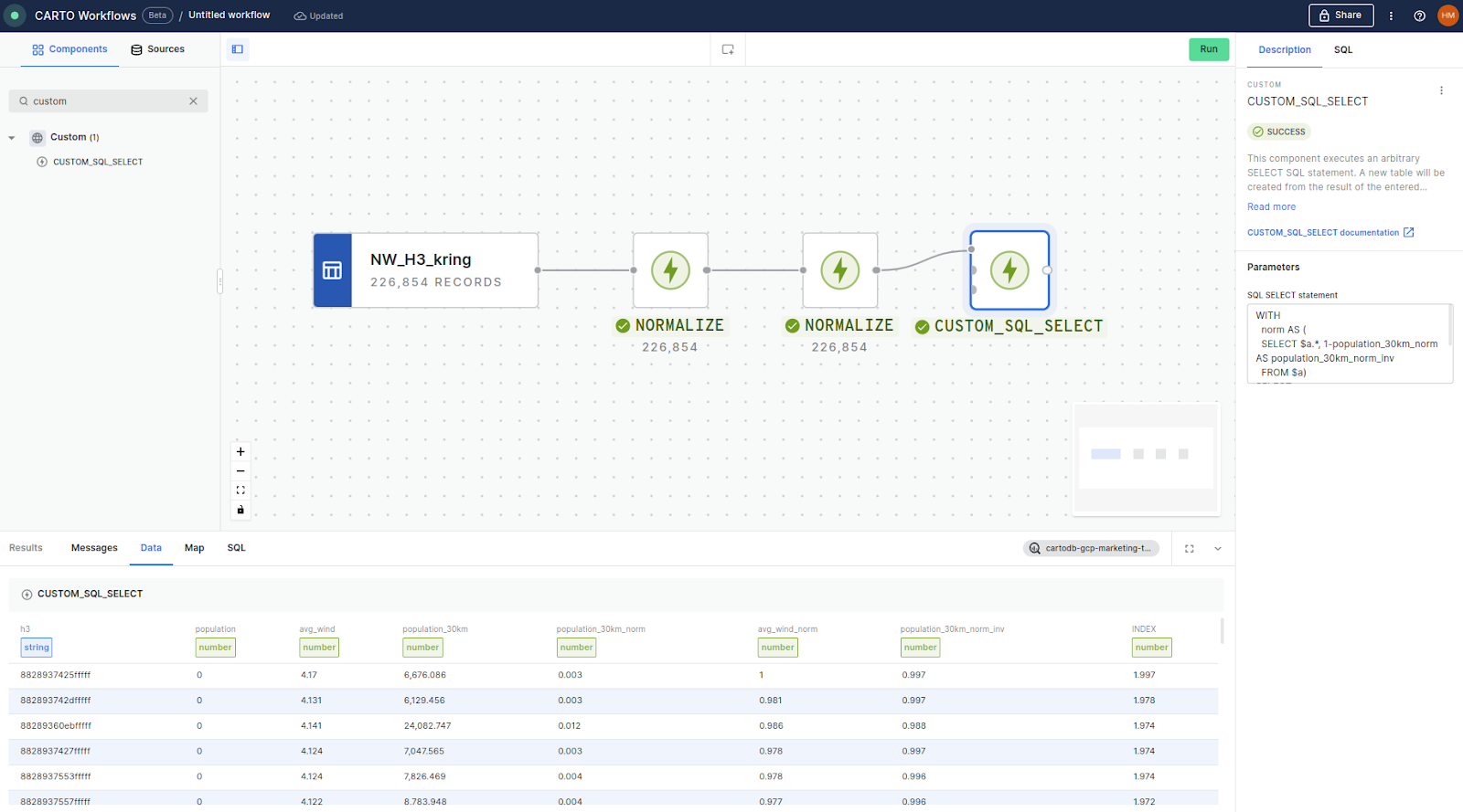
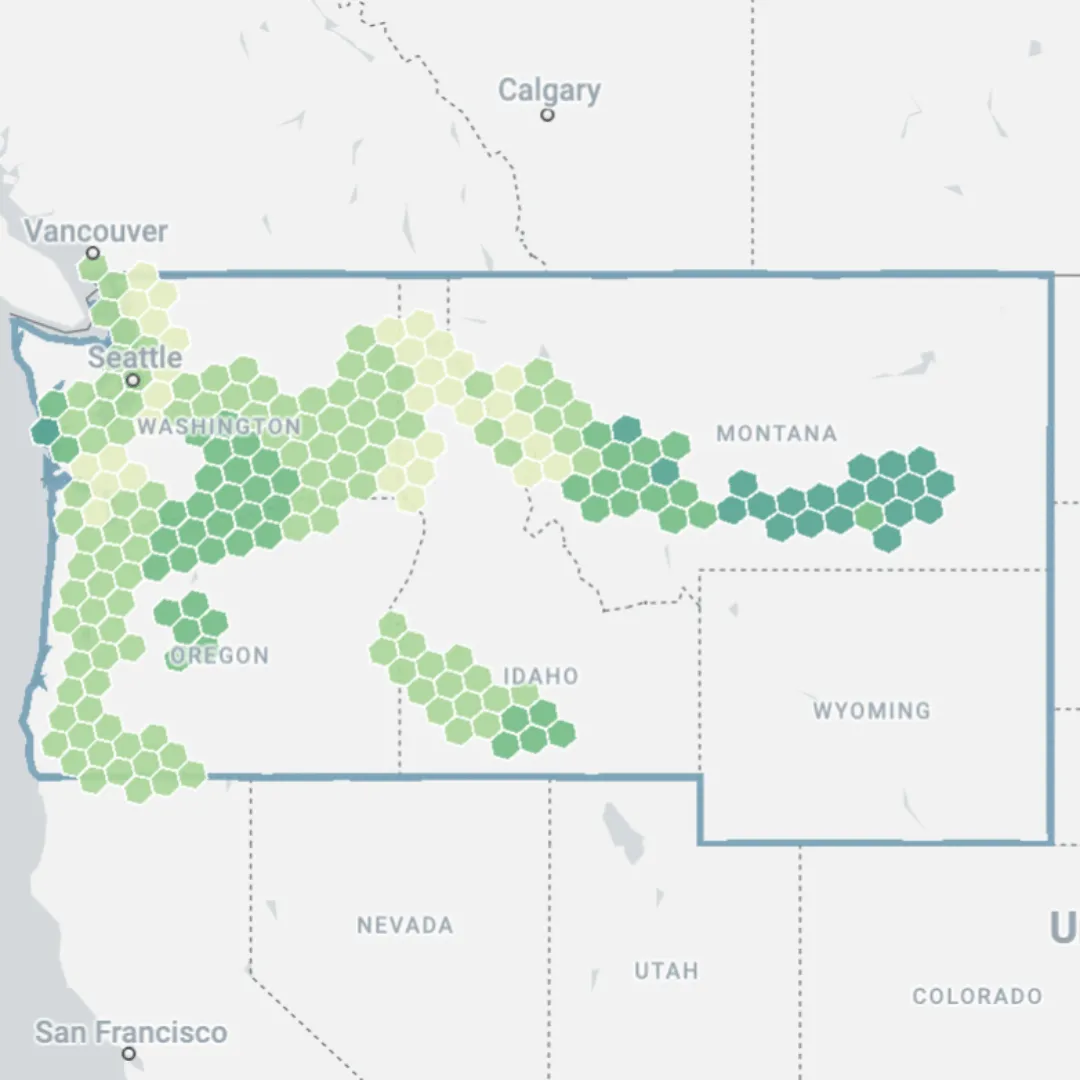
We just need to add two NORMALIZE components in order to - you guessed it - normalize each of our variables. Then finally - and this really is the final FINAL step - we add a CUSTOM_SQL_SELECT component. This SQL will inverse the population normalization (so the lowest population would score 1, as we would prefer our wind farm to not be located near a large population). It also adds the two normalization scores together to create a wind farm suitability index - with a maximum score of 2 indicating an area with the highest wind speeds and the smallest proximal population.
WITH
 norm AS (
 SELECT $a.*, 1-population_30km_norm AS population_30km_norm_inv
 FROM $a)
SELECT
 norm.*, population_30km_norm_inv+avg_wind_norm AS INDEX
FROM norm
Use SAVE_AS_TABLE again to export these results… and let’s check them out!
The results!
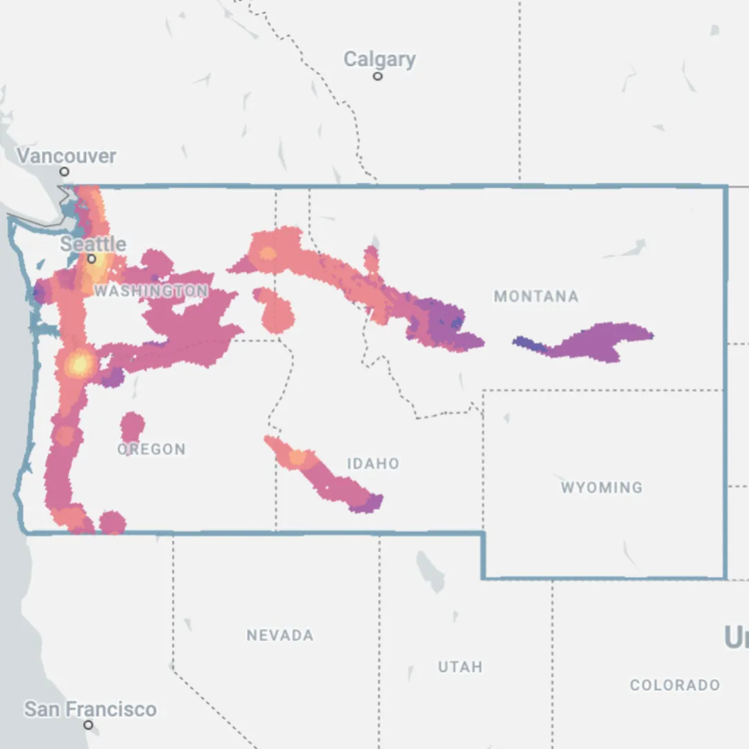
Access the interactive map here to see that areas of low suitability are more common to the west coast, around highly populated areas like Seattle and Portland. More suitable areas can be found particularly in the sparsely populated Central Montana, a state ranked 5th for potential wind energy power by the National Renewable Energy Laboratory. Wyoming is the only state where no suitable areas can be found, as there are no areas where the requisite power and transport infrastructure can be found in close proximity.
Location Intelligence for Renewable Energy Site Selection
This has been a simplified look at how different spatial datasets and analytical techniques can be used to pinpoint optimal locations for wind farms. Of course in reality, many more factors would contribute to this process - you can read more about using Location Intelligence for climate and environmental insights here.
Want to learn more watch this process in action in our mini-webinar below👇
Ready to see how you can using Location Intelligence to gain a competitive advantage? Make sure you grab a free two-week CARTO trial to give it a go yourself!


