Calculating Routes at Scale using SQL on BigQuery

Computing distance metrics is a challenging problem in spatial analysis. When studying urban travel, calculating distances between two locations as the crow flies is the most straightforward method but this approach often introduces gross errors. If we are after a more exact result, it is necessary to consider these distances as the shortest path taking into account the available transportation network.

We're excited to share the latest advancements from our Analytics Toolbox Routing Module - a cloud-native, scalable alternative to routing tools such as PgAdmin and ArcGIS Network Analyst. Our routing functions run directly inside Google BigQuery as part of our Spatial Extension, and can be further enhanced by using our curated data offering through the Data Observatory - also accessible through BigQuery.

Existing CARTO users may be familiar with the Routing Module of our Analytics Toolbox which we initially launched in August 2021. Since then, we’ve been optimizing and refining these tools and are excited to share the latest update! So what’s new?

You can read more details about what’s new with the Routing Module here.

Shall we try it out with an example? If you aren’t already a CARTO user, make sure you grab a free two-week trial so you can have a go yourself!

In this example, we’ll be imagining we’re a data analyst at a CPG company selling bottled drinks. Our fictional route-to-market is convenience stores, grocery stores and supermarkets across Nashville, Tennessee. 

Currently, our drinks are stored in a warehouse in the brilliantly named Pie Town area of Central Nashville. This used to be a fantastic location for quickly accessing our merchants, but traffic and rent increases are pushing us to move outside the city limits.

^{Routes from the existing warehouse to product merchants across Nashville.}

So, we need to understand which of our new warehouse options has the best location for accessing our merchants i.e. where are overall travel times the lowest.

Our potential warehouse locations have been extracted from the OpenStreetMap (OSM) Google BigQuery public dataset. This is a great resource for accessing data from what is often dubbed the “Wikipedia for maps.” If you’d like to know more about how you can leverage OpenStreetMap, check out our ultimate guide to doing this here. 

Using this guide, we’ve queried all OSM buildings with the tag “warehouse” within a 10-mile radius of Davidson County, Tennessee. The county boundary is freely available on our Spatial Data Catalog. We then created a 10-mile buffer around this using ST_BUFFER() and extracted the warehouses inside using the predicate ST_CONTAINS(). If you’d like to know more about how you can leverage Spatial Filters like this to streamline your analysis, check out our guide here.

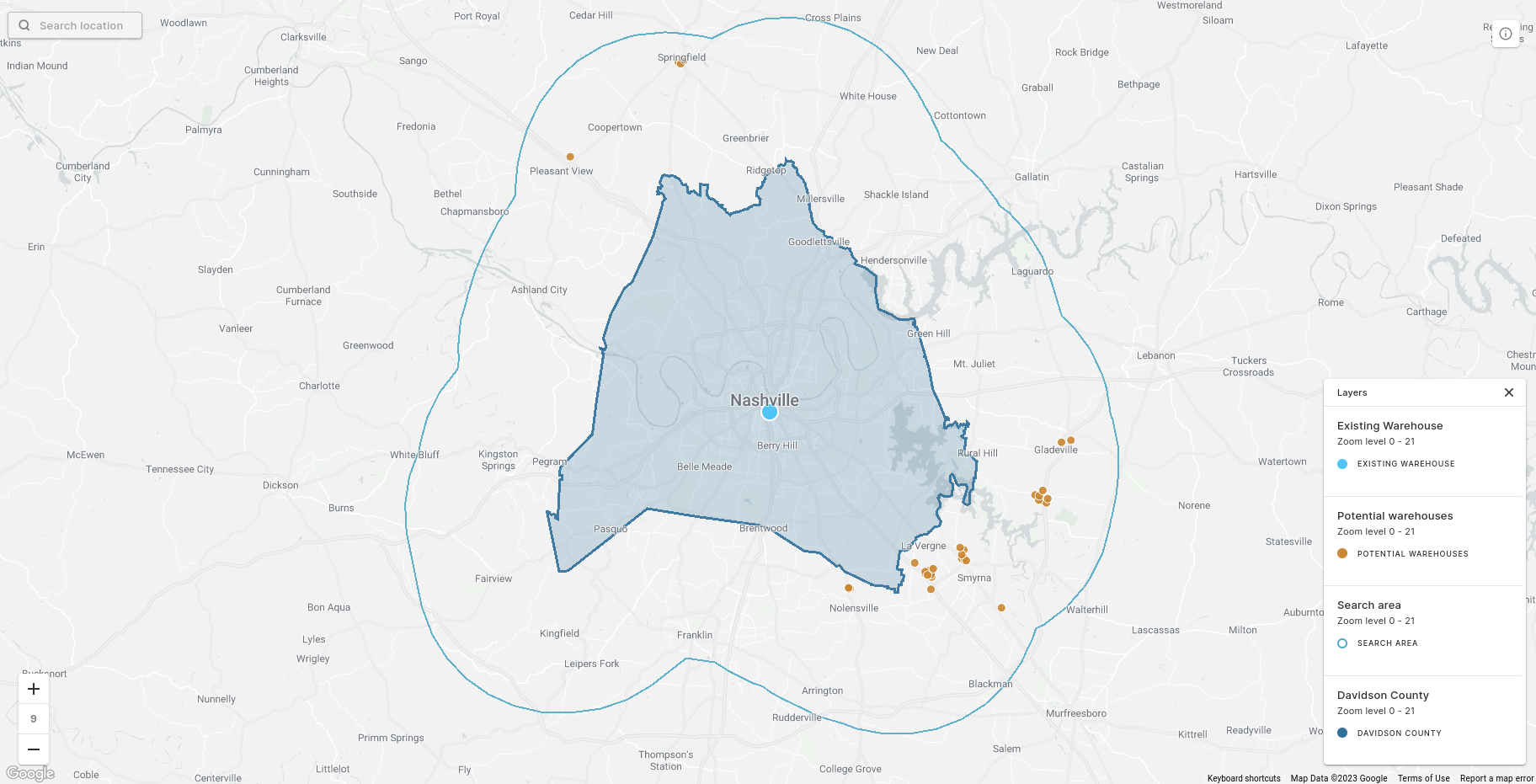
Now we can get started with the new routing tools!

You can run the Routing Matrix with a quick bit of Spatial SQL. It looks much more complex than it actually is!

   
  DECLARE origins ARRAY;
DECLARE destinations ARRAY;


-- Set start locations: warehouses in our search area
SET origins = (
   SELECT ARRAY_AGG(geom) AS origins
   FROM `yourproject.yourdata.osm_warehouses`
);


-- Set end locations: merchants in Davidson County
SET destinations = (
   SELECT ARRAY_AGG(geom) AS origins
   FROM `yourproject.yourdata.osm_merchants`
);


-- Run the routing matrix
CALL `carto-un.carto.ROUTING_MATRIX`(
-- Start locations
origins,
-- End locations
destinations,
-- Area to limit the calculations to
ST_BUFFER(ST_GEOGPOINT(-86.775411,36.150654),45000),
-- Transportation mode; car, car_motorways_only, bike, walk
'car',
-- Your network ID in the Data Observatory
 "cdb_road_networ_xxxxxxxx",
 --Your Data Observatory project & dataset
 'carto-data.ac_xxxxxxxx',
 --output_table
 'yourproject.yourdata.routing_potential',
-- Options; cost type, maximum cost, whether you wish to compute the geometry of the route
"""
{
   "TYPE":"time",
   "MAX_COST":"100000",
   "WITH_PATH":"True"
}
"""
) 
   

For a full explanation of this code and to understand all of the options available, check out our Documentation. 

You could even plug this into CARTO Workflows as a Custom SQL component and make this analysis part of a wider automated process!

The speed this will run at will depend on:

• The number of origins and destinations
• The size of the area you are calculating within
• The transportation mode; “car_with_motorways” includes the fewest links and so will be the quickest to run. Conversely, the walking network will be the most detailed and will take the longest time to compute. 

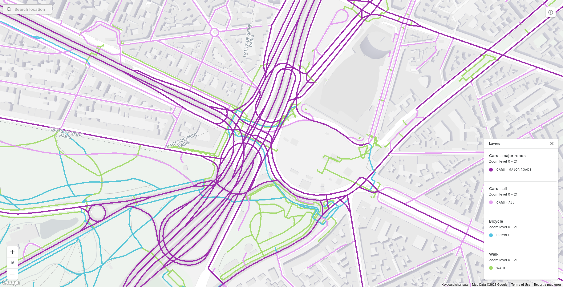
You can find your Data Observatory project, dataset and road network ID in your CARTO Workspace under Data Explorer > Data Observatory > CARTO > Road Network (you’ll need to have subscribed to this dataset to be able to see this - which is free to all users!). You’ll see your road network ID just under the table title, and can find your DO dataset & table by clicking “Access in.”

Once run, open up CARTO Builder add a custom query in to your map:

   
SELECT path AS geom FROM yourproject.yourdataset.routing_potential
   

And you should be able to see the results look something like this!

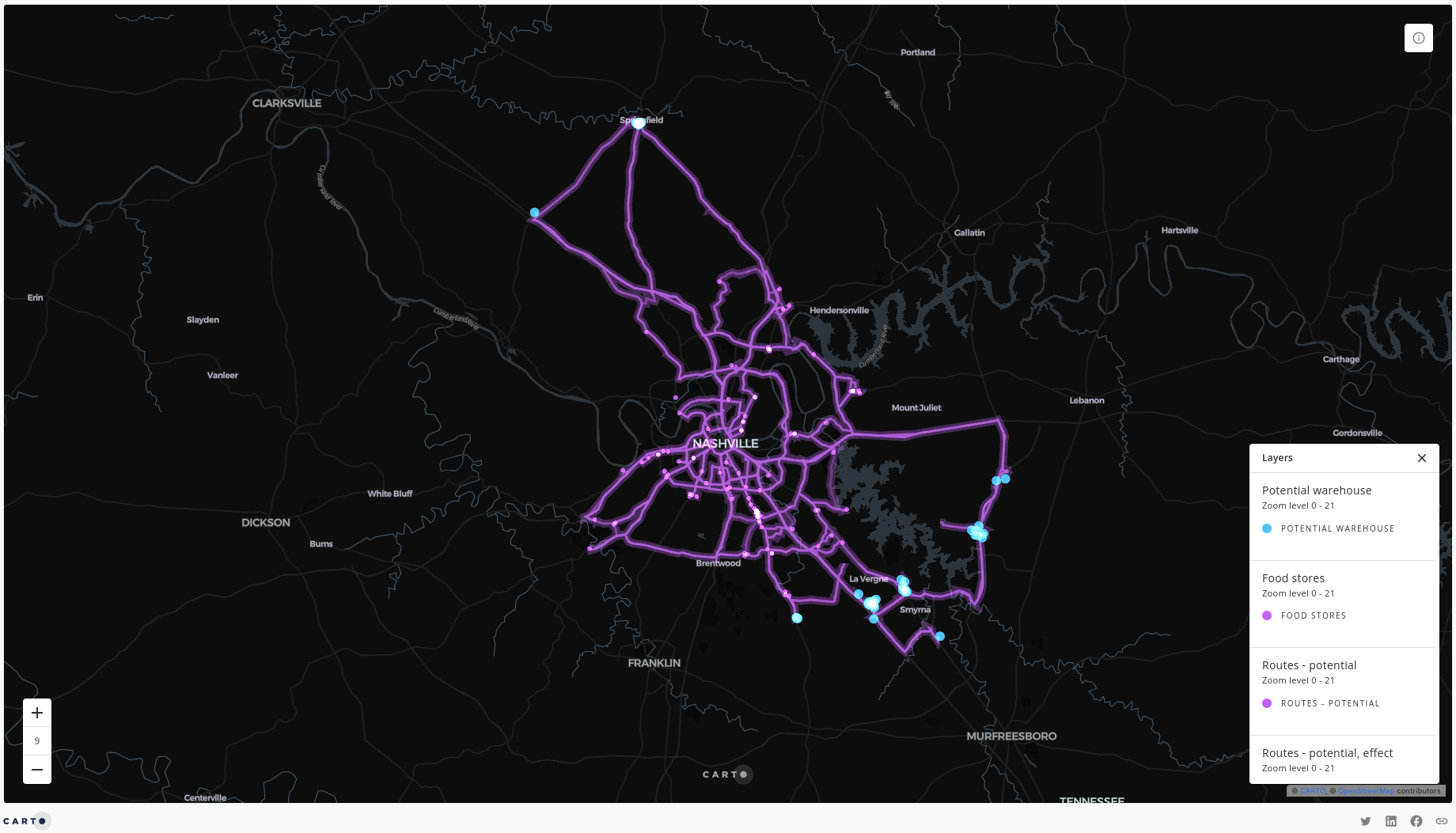
Really cool, but not actually an answer to our question.

A really simple way of establishing this is just by calculating the total distance a vehicle would have to travel from each warehouse, to each merchant. As well as calculating this, we can also take advantage of some of CARTO Builder’s dynamic visualization tools to help us to understand this.

We’ll need to join some of the data from our input warehouse table to our resulting table. This is always great practice in any spatial analysis as it will help you understand the “why” behind your results. We’ll also need to undertake a bit of post-processing:

   
WITH
warehouses AS (
 SELECT ST_ASTEXT(geom) AS geomtext, 
 CAST(ROW_NUMBER() OVER() AS STRING) AS warehouse_id 
FROM yourproject.yourdataset.yourtable)


SELECT
 ST_SIMPLIFY(paths.geom,5) AS geom,
 warehouses.warehouse_id,
 CAST(row_id() OVER() AS STRING) AS path_id,
 ST_LENGTH(paths.geom) AS length
FROM yourproject.yourdataset.routing_potential
LEFT JOIN warehouses
ON ST_ASTEXT(start.geo) = warehouse.geomtext
   

This code:

1. Adds an ID to each warehouse and each route feature - we’ll also cast this as a string field for us to be able to take advantage of some of Builder’s best visualization features! 
2. Calculates the length of the potential routes. 
3. An optional step here is to run ST_SIMPLIFY() on your geometry, as the paths created can often be very complex and therefore slow to render - we’ve simplified this to 5 meters.
4. Convert both the warehouse geometry and “start_geo” from the routing table to string using the ST_ASTEXT() function in order to…
5. Join the two tables together; we now have a “Warehouse_ID” column attached to our potential routing table..

Next, head over to CARTO Builder and add this table as a layer!

To find our optimum new warehouse location, we’ll be making use of the Category widget. This widget creates what is essentially a dynamic bar chart by grouping your data by a string field (hence why we needed a warehouse ID in the previous step), and aggregates numerical variables.

Here’s how:

1. Open the widget panel (top left of the Builder window)
2. Add a widget and select the routing results table which contains the post-processing from the previous step
3. Change the type to Category and the operation to SUM
4. Change the grouping field (the first one after operation) to the warehouse ID, the aggregation column to the route length, and the unique ID to the route ID. 

You’ll see a widget has now been generated with the 5 warehouses which have the highest total distance to travel to every merchant - but we’re interested in the least. Click “search all elements” and scroll right to the bottom, selecting the item with the lowest number.

This is our ideal warehouse! The total distance from here to all merchants is the lowest; you’ll see these now filtered on the map, all routed from “warehouse 41.”

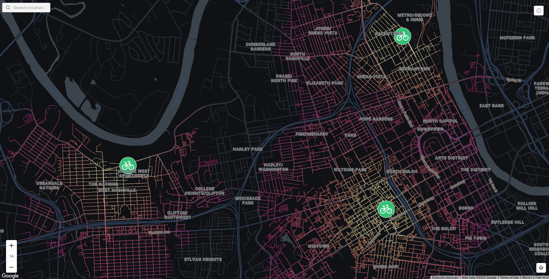
This is just a taste of the possibilities the routing module can help you unlock. For instance, you might decide that the driving distances from an out-of-town warehouse are too high, and you’d like to take advantage of a last-mile delivery microhub. As part of this process, you might want to use the ROUTING_ISOLINES function to work out which parts of the city are accessible within a specified cycling time.

We can’t wait to see how you use this module - make sure you sign up for a two-week free trial to get started today!

Want to get started?

Sign up for a free 14-day trial