Site Planning for Market Coverage Optimization with Mobility Data

In recent years the number of brick-and-mortar stores facing closure has swelled. In the retail sector this phenomenon has come to be known as the retail apocalypse but other sectors like banking are also being affected. However this retail apocalypse is not affecting all retailers and some online retailers have even announced plans to open their first physical stores. In this context it is more important than ever to consider cannibalization in both cases when deciding which stores to keep or close and when deciding where a new store should open. Spatial Data Science techniques are key to making a difference in tackling this challenge.

In this blogpost a case study is presented in which a bank is interested in expanding in the provinces of Sevilla Cádiz and Málaga in the south of Spain. Given their economic and business circumstances they are only planning on opening 10 branches and they would like to find locations where those branches can be accessible to as many people as possible. Therefore the focus of our work will be on identifying the 10 locations that attract the largest number of visitors while minimizing the potential cannibalization between branches. Human mobility data is a core component of our methodology.

This case study presents two main difficulties:

• Calculating the catchment areas for locations for which we are lacking historical customer data. Having these catchment areas is essential for modeling the potential cannibalization between branches.
• Identifying the optimal locations. This is a combinatorial optimization problem which means it is computationally hard to solve even for small instances.

The methodology developed in order to identify the 10 optimal locations is described in detail in the next sections. The main steps followed are:

1. Data discovery to identify relevant data for this case study.
2. Support (grid) selection and cell enrichment with the data identified in the discovery phase mainly human mobility sociodemographics and commercial data.
3. Catchment area calculation for a selected subset of cells. This subset of cells is obtained by applying a filter for identifying cells with high commercial potential. For this step we will use the methodology based on human mobility data explained in this previous blog post.
4. Optimization algorithm to identify the 10 best locations. An approximation algorithm is developed using a greedy approach and Linear Programming on every step of the algorithm.

1. Data Discovery

For data discovery we take advantage of the location data streams available in CARTO's Data Observatory and the enrichment toolkits available in CARTOframes so that we can easily bring in features from human mobility socio-demographic financial and other data categories.

Since bank branches have higher utilization in places with higher footfall and where the commercial activity is high we identified the following data as relevant:

• Human mobility: footfall and origin-destination matrix (source: Vodafone Analytics)
• Points of interest (source: Pitney Bowes)
• Commercial intensity indices (source: Unica360)
• Sociodemographics and socioeconomic data (source: Unica360)

The following dashboard shows some of the data used. To learn more about the location data streams that CARTO offers please visit our Location Data Streams Catalogue

.

2. Support Selection and Cell Enrichment

The base of our method is the use of human mobility data from Vodafone Analytics. Therefore we selected Vodafone's 250m x 250m cell grid as the reference grid to project all the other features.

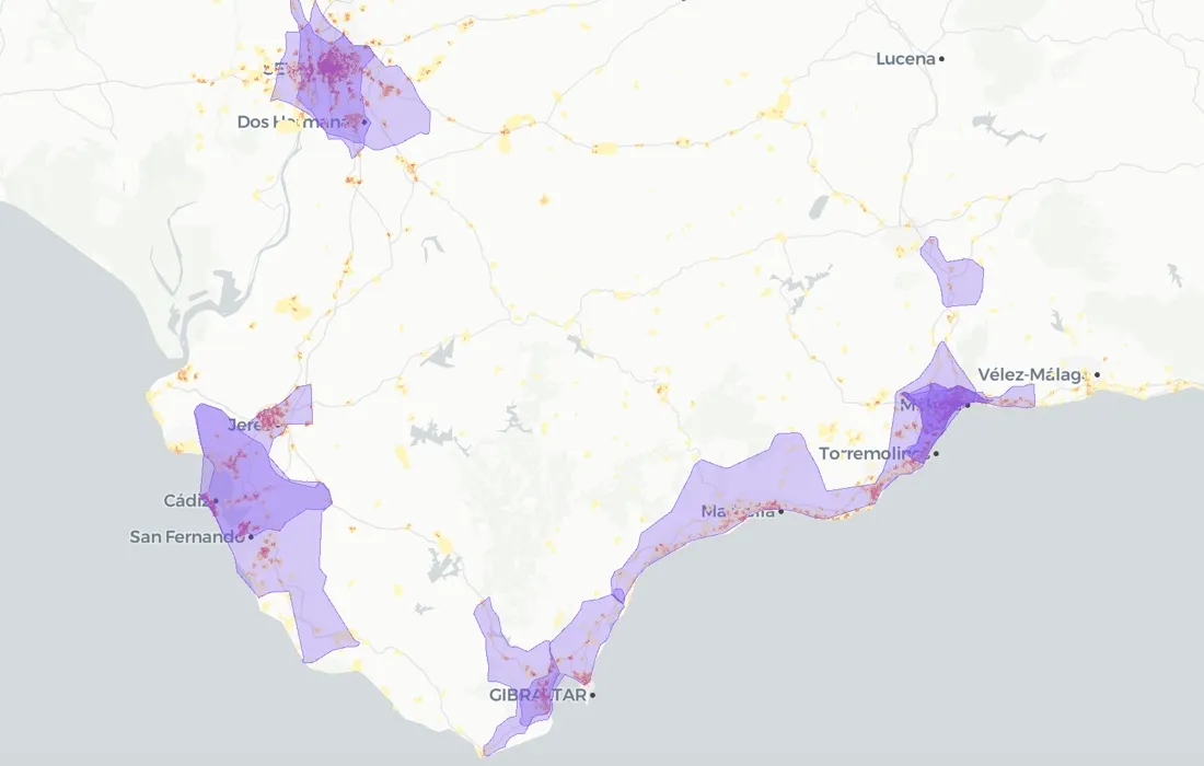
On the following map you can visualize the grid and the focus area (Sevilla Málaga and Cádiz).

Fig 1. This map shows the focus area and the candidate cells

We enrich the grid as described in the following sections:

Human Mobility Data

Vodafone Analytics data provides insights on the number of people visiting any 250m x 250m grid cell covering the entire territory of study. Vodafone anonymises aggregates and then extrapolates the data measured in the network to provide insights representing the overall national and international population. In addition this data also provides the origins of the visitors aggregated at different levels depending on the distance to the destination cell.Cells are enriched with the following data from this source:

• Total number of visitors
• Total number of visitors by origin and activity
• Average number of visitors in the cells within a buffer from the cell's centroid

Fig 2. This choropleth map shows the normalized number of visitors coming from every origin to a destination cell in the city of Sevilla.

Commercial Activity Data: Points of Interest (POIs)

This dataset provides information on POIs. Cells are enriched with the following data from this source:

• Number of competitors within a 250 meter buffer from the cell's centroid.
• Number of POIs within a 250 meter buffer from the cell's centroid. Here we use POIs as a proxy to commercial activity.

Commercial Activity Data: Commercial Indices

This dataset provides some commercial indices (general retail health care etc.) consisting in normalized commercial activity values ranging from 0 to 1; 0 being very low commercial activity and 1 being very high.

Cells are enriched with the following data from this source:

• General commercial index
• Hotel business index
• Retail index
• Public transport index
• Healthcare index

Sociodemographic and Socioeconomic Data

This information is provided on a 100m x 100m cell grid. The data aggregation is upscaled to fit the 250m x 250m cell grid applying areal interpolation.Cells are enriched with the following data from this source:

• Population
• Average household income
• Amount of people working at the target cell

{% include icons/icon-bookmark.svg %} Looking to add more skills to your Spatial Data Science toolkit? Our free ebook can help!

3. Filtering and Building Catchment Areas

Once the grid is enriched and before calculating the catchment areas we reduce the search space by applying a filtering step so that only cells with high commercial and economic potential are considered for opening the branches.

The filtering uses the following criteria with predefined thresholds on each of them:

• Number of visitors within a 250 m buffer from the cell's centroid. This minimum is increased in the presence of competitors within that same buffer.
• Number of POIs within the 250 m buffer.
• Retail intensity index.
• Average household income.
• Number of people working in the target cell
• Population

After analyzing different scenarios with different thresholds and visualizing them to check everything made sense based on our knowledge of the focus region we set the following cuts on these six criteria.

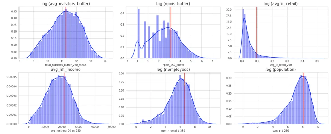
Fig 3. Thresholds applied for the filtering. The plots show the distribution of the criterion variables and the selected threshold for each of them. Note log transformation has been applied to some distributions.

As a result we reduced the search space from more than 18 000 initial cells to 620. The following figure shows all grid cells in the area around the city of Sevilla on the left and the remaining cells after filtering on the right.

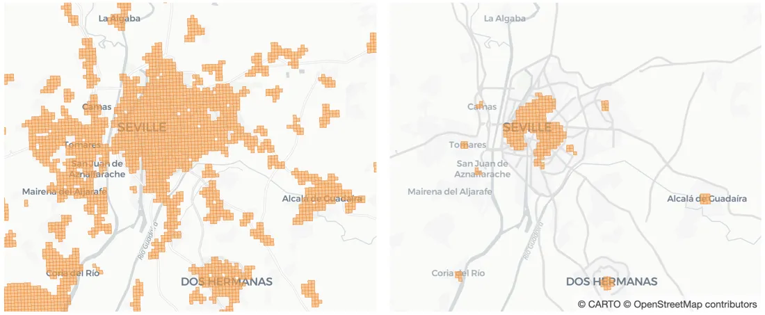
Fig 4. On the left the reference grid in the area around the city of Sevilla. On the right the remaining cells in the same area after filtering.

Finally catchment areas are built using human mobility data and following the methodology presented in this previous blog post.

4. Location-allocation. Optimization

Location-allocation is the name given to a set of optimization algorithms focused on identifying the best placements for facilities to serve a collection of demand locations. They have been extensively used in various sectors such as Logistics to find the optimal locations for distribution centers Retail to find the optimal location to open new stores and Telco to find the optimal locations to install antennas.

The case study presented here is also a good example of a location-allocation problem where a bank is interested in finding the 10 locations to open new branches from which they can reach out to as many people possible. This implies finding the locations with the highest number of visitors while minimizing the intersections between their catchment areas because visitors will only be counted for one of the locations. These intersections between catchment areas will be considered as the potential cannibalization between pairs of locations.

This specific case of the location-allocation problem is known as the Maximum Coverage Problem (MCP). We have an important difference to the standard MCP though since in our case a specific origin can have (and most times does have) a different number of visitors going to different destination cells.

Location-allocation problems are combinatorial optimization problems well known for being very hard to solve even for small instances. This is because the number of possible solutions increases exponentially with the number of candidate locations to be considered and the number of optimal locations to identify. The table below shows the number of possible solutions depending on the number of optimal locations we are interested in finding among the 620 candidates we have:

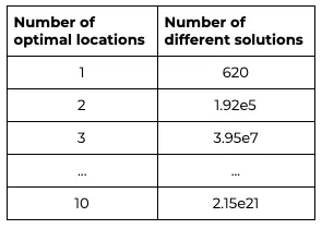
Table 1. This table shows the number of different solutions of the location-allocation problem for 620 candidates depending on the number of locations to be selected.

Because of the high combinatorial complexity of the MCP problems approximate algorithms are commonly used leaving exact algorithms only for small instances of simplified versions of the problem.

The most frequent approach followed in literature are greedy algorithms followed sometimes by some local search heuristic to make sure the nearest local optimum is reached. Some more advanced metaheuristic algorithms have been designed to be able to escape local optima but their complexity increases with the number of concurrent swaps allowed at each iteration. Therefore most times these more advanced approaches have only been tested allowing one swap per iteration which makes it harder to explore distant areas within the solution space.

The Algorithm

The algorithm we have designed to solve this problem follows a greedy approach using Linear Programming at every iteration to improve the chances of finding better local optima. A single-swap local search heuristic is applied on the solution found to make sure we are at a local optimum.

You can read more about Linear Programming in this previous post.

Initial Consideration

The algorithm is designed using a simplification of the problem based on the fact that having an origin within three catchment areas of the selected locations is worse than having an origin within two catchment areas (i.e. more potential cannibalisation). More generally speaking having an origin within n catchment areas of the selected locations is worse than having an origin within n-1 or fewer catchment areas.

This fact allows us to solve the problem considering only pairwise intersections which notably reduces the complexity. The total number of potential customers covered by the 10 selected locations is calculated adding the visitors of every catchment area independently and subtracting the double-counted visitors in every pairwise intersection. This calculation assigns an increasing penalty for having an origin polygon within several catchment areas proportional to the number of catchment areas containing the polygon.

The following example aims at showing the difference in the calculation of potential customers when calculating with and without the just described property. In this example we have three selected locations their catchment areas and the intersections between them.

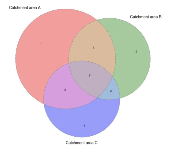
Fig 5. This Venn Diagram represents the different possible intersections among three catchment areas.

The number of potential customers would be calculated as follows:

• Not using the property: Number of visitors coming from each of the three catchment areas minus visitors coming from 5 6 and 3 (because they should only be counted once) minus two times (2x) visitors coming from 7 (because they are in the intersection of the three but should be counted only once).
• Using the property: Number of visitors coming from each of the three catchment areas minus visitors coming from 5 6 and 3 (because they are within one pairwise intersection) minus three times (3x) visitors coming from 7 (because they are within the three pairwise intersections).

Algorithm Description

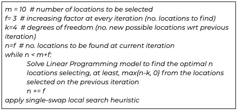
As mentioned above we follow a greedy approach applying Linear Programming at every iteration. The greedy algorithm consists of selecting 3 new locations at each iteration allowing for one of the locations selected on the previous iterations to be changed (i.e. allowing one swap). Below you can find the pseudocode of this greedy algorithm:

The Linear Programming model solved at each iteration is presented below.

The Linear Programming model is solved using Google OR-Tools a powerful optimization solver wrapper that allows to connect to a wide range of commercial and free solvers.

In order to improve the efficiency of the algorithm we define variables $$X_{jk}$$ as continuous and we only penalize those pairs of locations whose intersection contains more than 10% of the visitors from both locations. Further improvements could be achieved by:

• Calculating an initial solution (with a purely greedy approach for example) and:
  (a)Using it as a warm start.
  (b)Using the number of visitors of the location with the lowest number of visitors as a lower bound for the Linear Programming model.
• Applying some local search heuristic after each iteration of the greedy algorithm.

Results

After running the optimization algorithm for different values of f (increasing factor) and k (degrees of freedom) we obtain the solution shown on the map below. The total number of potential customers for the best solution we obtained is 3 223 552.

The following map shows the selected locations and their catchment areas.

Fig 6. Map with the 10 locations selected for opening new bank branches and their respective catchment areas.

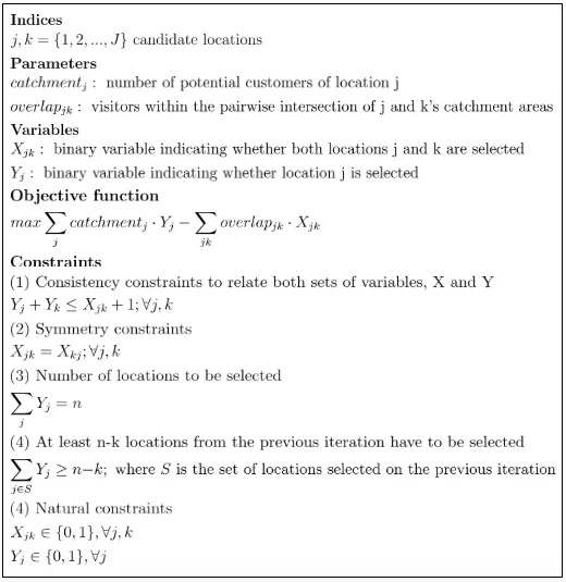
If we analyze what municipalities are covered by the catchment areas of the locations selected by the CA (see figure 7 below) we can see all municipalities with a population over 50 000 people are at least within one of the location's catchment areas. In addition it can be observed that the larger the population of a municipality is the greater the number of catchment areas covering them.

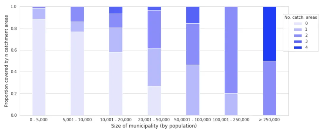
Fig 7. Proportion of municipalities by population range covered by 0 1 … 4 catchment areas

In order to assess the quality of the algorithm developed at CARTO (CA) we'll compare the results obtained using our algorithm with the standard greedy algorithm (SGA) that is usually used to solve the location-allocation problem. The SGA finds one new location at each iteration and updates the number of potential visitors of non-selected locations considering the intersections with the already selected locations. This algorithm does not allow swapping.

The number of potential visitors covered by the catchment areas of the locations selected by the SGA is 2 884 347. This means CA is able to improve this result by almost 340 000 visitors which represents an extra 11.75% visitors.

The map below shows the catchment areas of the locations selected by both algorithms. These areas are plotted over the reference grid colored by the number of visitors at each cell. The main difference that can be observed is that some of the catchment areas of the locations selected by the SGA are larger and cover areas with a lower population density which implies lower quality locations. This is because after the first 5-7 locations are identified some swap is needed in order to find new good quality locations. However the SGA does not perform any swapping.

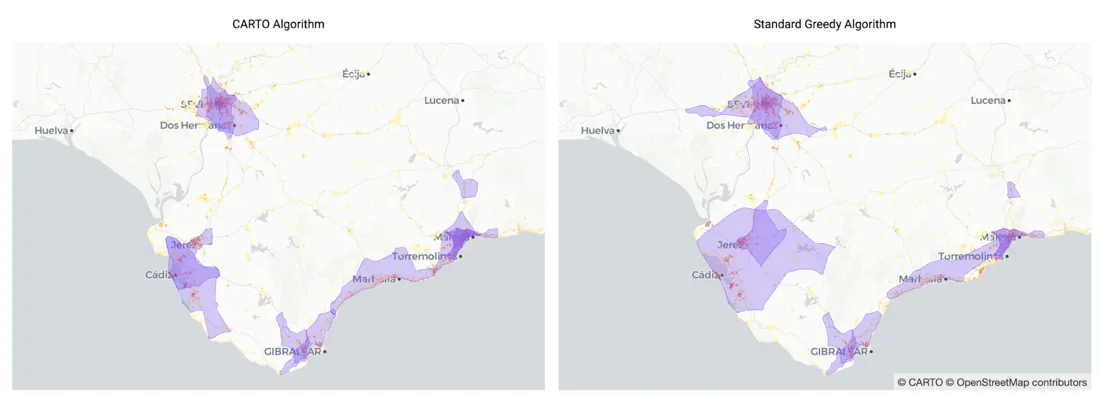
Fig 8. Map showing the catchment areas of the 10 locations selected with the algorithm developed at CARTO (left) and the Standard Greedy Algorithm (right) over another layer with the candidate cells colored by number of visitors.

Further steps: Calculating the optimal number of locations

In this blog post we have presented a site selection case study in which the number of new bank branches to be opened was known beforehand. Often times companies find it very hard to come up with this number. The methodology presented here can also be used to answer this question with a small change in the optimization algorithm developed.

Here it is essential to know what criteria is going to be used to determine the optimal number of locations. One possible criteria could be market saturation. Market saturation can be defined as a threshold such that if the number of new potential customers covered when one new location is added is below that threshold market saturation is reached..

For example for a 5% threshold we have that the optimal number of locations is 10 as can be seen in the figure below.

Fig 9. Increase in number of potential customers by increase of new locations. Threshold of 5% for market saturation.

The algorithm developed at CARTO (CA) presents a better performance than the SGA for this problem as well. Below we can see the number of potential customers covered depending on the number of locations selected. We can see for a low number of locations both algorithms have a very similar performance and as the number of locations increases (and hence the problem gets harder to solve) CA performs better than SGA. This means SGA will reach a saturation point before CA missing market potential.

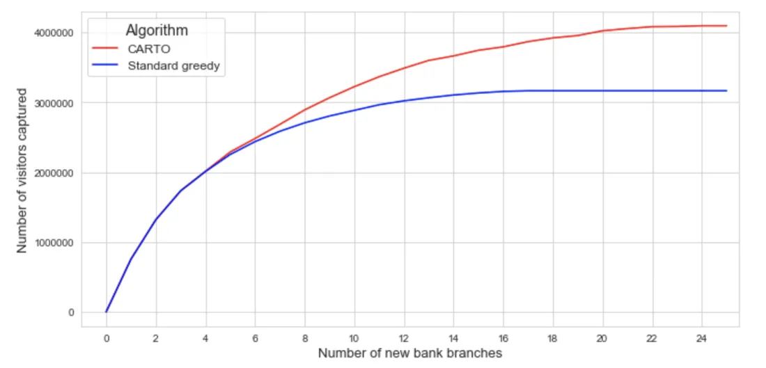
Fig 10. Number of visitors covered by both algorithms depending on the number of new locations.

In particular we can see CA can perform up to 30% better than SGA depending on the threshold set for market saturation.

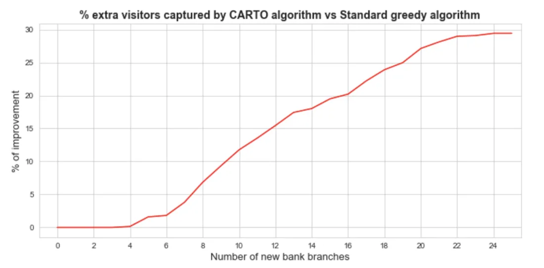
Fig 11. Performance improvement of CA vs SGA.

Conclusion

Today's challenging context affecting retail and other sectors makes it imperative for them to use the techniques and tools that will allow them to make informed decisions and stand out from their competitors.

Human mobility data enriched with other data streams and the use of optimization and other spatial techniques will make a difference when tackling the challenges these sectors are facing today and the ones to be faced in the future.

Special thanks to Mamata Akella CARTO's Head of Cartography for her support in the creation of the maps in this post.