How to use Location Intelligence to grow London's brunch scene


Things Londoners love: tube etiquette, avoiding Oxford Street, and brunch! Whether it’s decompressing from the week over an almond croissant, or recalling (or not) the night before over a full-english - England’s capital is brunch-obsessed.
London has also seen a rise in popularity of brunch deliveries, fuelled by pandemic and convenience driven-trends.
But with tables filling up - and the capital’s population set to grow by over one million in the next 20 years - this raises the question: does London have enough brunch spots? And if it doesn’t, where are more needed?
Let the investigation begin. Make sure to grab a free two-week CARTO trial to try this out yourself!

Where do Londoners love brunch?
Let’s start this investigation by establishing spatial patterns of brunch affinity across London.
Luckily, our Spatial Data Catalog contains a suite of data which does exactly that. Our data partner Spatial.ai’s dataset “Proximity” (currently available for the USA, UK & Canada) aggregates and classifies user experiences, personalities and feelings shared over various social media platforms. Areas are given a score against 72 different profiles based on how well they align with those profiles.
One such profile is “Breakfast and Brunch affinity.” Residents in an area scoring 99 love a flat white and avocado toast more than 99% of the rest of the country.
Let’s take a look!
Accessing the data
You can access Spatial.ai’s Proximity dataset in the Data Observatory panel of your CARTO Workspace by either accessing a sample or requesting a subscription.
As we’re only interested in London, we need to filter the data to this region. First, we need a geometry which describes the area of London. This can be easily sourced and loaded into your data warehouse from the Office for National Statistics here.
We can then perform a Spatial Filter (full guidance on how to do this here) to extract the data we’re interested in. This can be tricky as - if the zones don’t exactly align - our filter can be erroneous. Our experience has taught us that the safest thing to do here is to first convert the LSOAs to centroids (using the function ST_CENTROID), and then perform the filter.
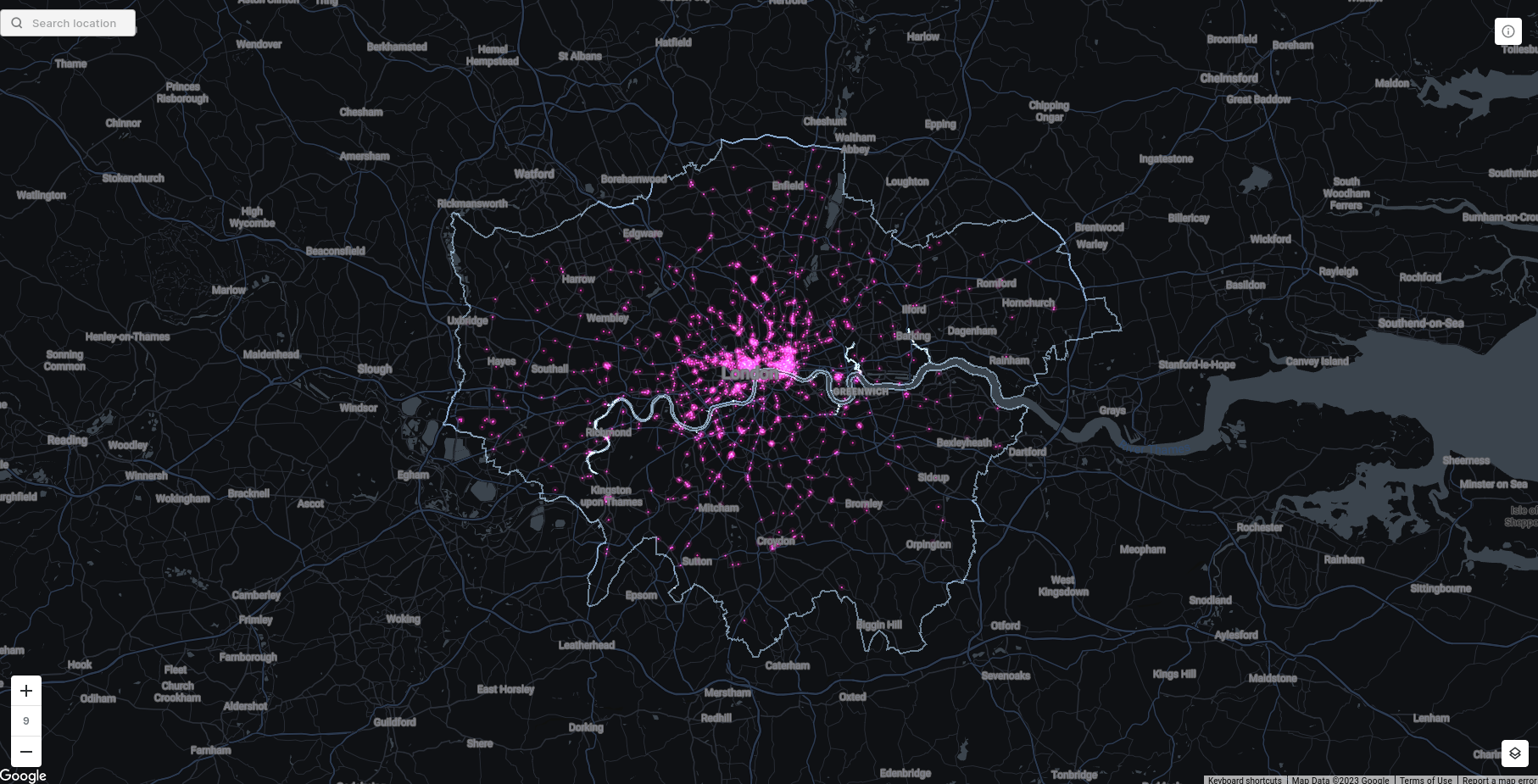
That gives us the following results, with darker areas being more partial to brunch.
Open this map in fullscreen here.
Apart from Central London being clearly brunch-obsessed, it’s actually pretty difficult to establish trends in this data from this map. This is because LSOAs are an irregular zonal geography, being sized and shaped to fit a roughly equal number of people in each zone.
The result of this is that visualizations are dominated by relatively sparsely populated areas, such as the suburban fringe or green spaces like Richmond Park. Conversely, the densely populated inner city is really difficult to see, as the zones are so small.
To draw conclusions from this, we need to first convert this data to a “regular” geography, and then establish the total target market.
Converting data to a regular geography
Spatial Indexes are perfect for this type of analysis.
These are global multi-resolution grid systems; what makes them special is that they aren’t geolocated like traditional geometries - with a long linestring describing the coordinates of every vertex - but with short reference strings. This makes them tiny to store, but - crucially - lightning fast for analysis like this. We love Spatial Indexes so much we’ve written a WHOLE ebook about how you can use them in your analysis - check it out here!
In addition to knowing our brunch affinity index, to be able to calculate the total target market, we’ll need to know the population of each Spatial Index cell. We’ll be using the free dataset Population Mosaics - United Kingdom (Grid 100m, 2020) as a source for this.
We can easily join this data to the H3 grid with our enrichment tools, specifically “Data Observatory - enrich grid.” This function is designed to aggregate data from our Data Observatory into Spatial Indexes. This is a really helpful tool, as you can join variables from any number of input datasets and variables, rather than having to make these aggregations source-by-source.
We’ll also use the function H3 Polyfill to generate a H3 grid across London.
CALL `carto-un`.carto.DATAOBS_ENRICH_GRID(
 'h3',
 R'''
   SELECT h3 FROM unnest(`carto-un`.carto.H3_POLYFILL(
   (SELECT st_union_agg(geom)
   FROM `my-project.my-dataset.regions`
   WHERE RGN21NM = 'London'), 9)) h3
     -- Input Spatial Index table or query
 ''',
 'h3', -- Index reference field
 [('population_c7e5d619', 'sum'),('index_breakfast_ebc42ec5','avg')],
   -- source variables
 NULL,
 ['my-project.my-dataset.my-enriched-table'], -- Output table
 'my-dataobs-project.my-dataobs-dataset'--Your data observatory dataset
)
The SQL code above - which you can execute either in your data warehouse console or a CARTO Workflows call procedure - will do this. You will need to know the IDs of your source variables, which you can find under the Data Explorer page for each input dataset.

You’ll also need to know your Data Observatory dataset name, which you can find in the Data Explorer when you click “Access in” to any Data Observatory table you’re subscribed to. It will look like “carto-data.ac_xxxxxxxx.”
This will result in a H3 grid with a field for both population and brunch affinity. For more information on data enrichment, check out our full guide.
Calculating the Total Addressable Market
In this instance, we’re going to calculate the Total Addressable Market (TAM) using the simple formula (Index/100)*population. This means that if an area with a population of 500 has an index of 100, then we will say 100% (i.e. 500 people) of the area’s residents are a target.
SELECT
*,
(index_breakfast_ebc42ec5_avg/100)*population_c7e5d619_sum AS market
FROM
My-project.my-dataset.my-enriched-table
Copy this query into CARTO Builder’s Custom SQL console - making sure to change the feature type to H3 - and explore the results! It should look something like the below:
Open this map in fullscreen here.
Where is there a brunch deficit?
So now we know where there is a strong market for brunch. Next, we need to compare that with the distribution of brunch spots.
To identify these, we’ll be using Safegraph’s Places dataset, which is available by premium subscription from our Spatial Data Catalog.
Once subscribed, you’ll see this dataset contains lots of useful information; from contact details to the date it opened. We’re really interested in the “category_tags” field. We can extract just the Places of interest using the LIKE operator and wildcards (“%”) to return locations where brunch is just one of the category tags - see below.
…WHERE category_tags LIKE ‘%Brunch%’
By also applying the regional Spatial Filter to only look at locations in London, we are left with 1,367 brunch locations.
Calculating the total target market
Before we get to delve into the results of this analysis, we need to calculate one final thing; the number of brunch spots within a distance of each H3 cell. If the total market is high but the number of brunch spots is low, we’ve found a prime location for brunch growth!
We’re going to assume that residents will travel a 15-minute walk for brunch, which is approximately 1,200 meters. We’ll just be using a fixed distance buffer to illustrate this, but for extra precision you could use 15-minute isolines to assess this.
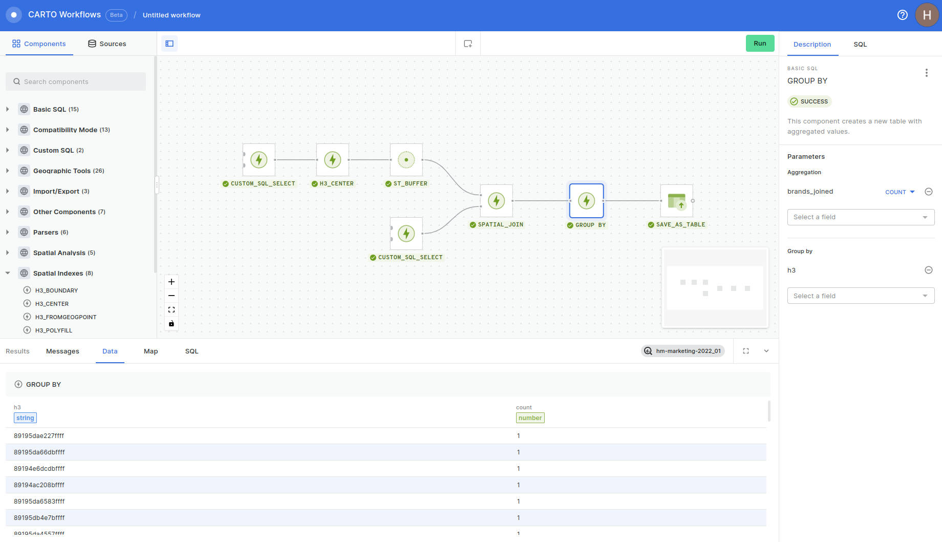
The steps which comprise this workflow are:
- CUSTOM_SQL_SELECT to select our H3 with the custom target market calculation
- H3_CENTER to create center points for each H3 cell.
- ST_BUFFER to create our 1,200 meter/15 minute walk buffers from each cell.
- CUSTOM_SQL_SELECT to select the Safegraph Places with the category tag “brunch.”
- SPATIAL_JOIN to join the brunch spots to the 1,200 meter buffers.
- GROUP_BY to count the number of spots in each buffer, grouped by the H3 ID column.
- SAVE_AS_TABLE to export this as a table.
This results in a table which contains:
- H3: the H3 reference column.
- TargetMarket: the population who we estimate love brunch in that cell.
- BrunchLocationCount: the number of brunch locations within a 15-minute walk.
The results!
Open this map in fullscreen here.
The results of this analysis are visualized in the Builder map above! By adding a couple of Range Widgets, we can filter the results to areas which have a high Total Addressable Market, but a low number of brunch spots within 15-minutes. This filters out a lot of low populated areas - such as Richmond Park - as well as areas dense with brunch spots, such as Central London, Islington & Clapham. But we’re also left with a lot of areas crying out for more brunch! These might be areas where a business could:
- Open a new location or franchise
- Place a ghost kitchen to enable more brunch deliveries
- Sign up more nearby brunch restaurants to a food delivery service
- Target marketing activities for brunch-themed meal kits
If you’re interested in hearing a real-world example of how Location Intelligence is helping companies fuel growth in food delivery, check out our Deliveroo customer story here. You can also watch the creator of this analysis Helen McKenzie walk through this analysis at Big Data LDN 2022 here.
Has this post given you a taste for Location Intelligence? Pick up a free two-week trial today!